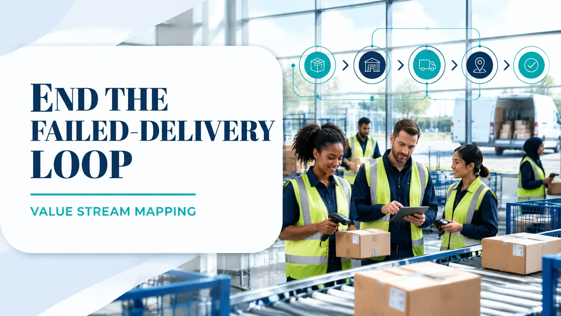
In last-mile delivery, the customer experiences one outcome: a parcel arrives on time, intact, at the correct address, with reliable proof of delivery. Behind that outcome sits a complex stream of parcels, scans, route decisions, vehicle movements, customer notifications and delivery attempts.
Value Stream Mapping (VSM) makes that stream visible. The material flow is the movement of parcels through the depot and delivery network. The information flow is the sequence of scan events, route manifests, address data, driver instructions, exception codes and customer notifications.
When these flows are mapped together, delivery leaders can see where time is added, where work waits, where defects originate and why a failed delivery creates a costly loop through redelivery, customer contact and additional depot handling.
This guide presents a practical VSM for a hypothetical parcel depot processing 12,000 parcels per day across 60 delivery routes.

1. Select the Mapping Boundary
The mapping boundary should follow the parcel from the point at which the depot accepts operational responsibility through to successful proof of delivery or a controlled redelivery path.
In scope
- Depot inbound unload and arrival scan
- Primary sortation
- Secondary sortation to delivery route
- Route allocation and manifest generation
- Vehicle load-out
- Driver departure and road delivery
- Delivery attempt
- Proof of delivery
- Failed-delivery coding
- Redelivery booking and next-attempt preparation
Outside scope
- E-commerce order processing and customer picking
- Supplier packaging before line-haul arrival
- Long-distance line-haul network design
- Customer refunds and claims after delivery
- Full reverse logistics after a parcel is formally returned
The boundary is deliberately narrow enough for a focused improvement project while still capturing the failed-delivery loop, which often crosses depot, driver and customer-service functions.
2. Current-State Walkthrough: A 12,000-Parcel Depot
Assume the depot receives 12,000 parcels daily. With 60 routes, the average route load is:
12,000 parcels ÷ 60 routes = 200 parcels per route
The depot operates a 10-hour processing window. Therefore, the network takt at depot level is:
600 available minutes ÷ 12,000 parcels = 0.05 minutes per parcel, or 3 seconds per parcel
This does not mean one employee must process a parcel every three seconds. It establishes the required system rhythm across all parallel resources.
Current-state process data
| Process step | Typical current-state measure |
|---|---|
| Inbound trailer unload and scan | 45 minutes |
| Primary sortation cycle | 70 minutes |
| Wave wait before secondary sort | 90 minutes |
| Secondary sortation cycle | 95 minutes |
| Route allocation wait | 55 minutes |
| Run sheet generation | 15 minutes |
| Vehicle load-out | 75 minutes |
| Average depot dwell | 8 hours |
| On-road hours available | 8 hours |
| Average stops per route | 160 |
| Stop density | 20 stops per route hour |
| Average drive time between stops | 1.8 minutes |
| Average service time at stop | 1.2 minutes |
| First-attempt delivery rate | 92% |
| Failed-delivery/card rate | 8% |
| Average redelivery delay | 24 hours |
For the delivery portion, each route has 160 stops and 200 parcels. The route therefore carries an average of 1.25 parcels per stop.
The route rhythm is:
160 stops ÷ 8 hours = 20 stops per hour
Each stop consumes approximately:
1.8 minutes driving + 1.2 minutes service = 3 minutes
That equals:
160 stops × 3 minutes = 480 minutes, or 8 hours
The route is therefore fully loaded. Any delay at load-out, address correction, customer access or proof-of-delivery capture reduces the available delivery capacity.
Lead time and process cycle efficiency
A parcel that arrives at the depot at 10:00 p.m. may not reach the customer until the following afternoon. A representative successful parcel has:
- 8 hours depot dwell
- 8 hours on-road delivery time
- Approximately 16 hours from inbound scan to proof of delivery
The failed-delivery loop increases average lead time. With an 8% carded rate and a 24-hour redelivery delay:
- Successful parcels: 92% × 960 minutes = 883.2 minutes
- Failed parcels: 8% × 2,400 minutes = 192 minutes
- Weighted average lead time: 1,075.2 minutes, or approximately 17.9 hours
Assume customer-required value-added time per parcel includes:
- Sort and scan handling: 0.6 minutes
- Allocated share of loading and delivery work: 3.0 minutes
- Delivery handoff and proof of delivery: 0.6 minutes
Total value-added time is 4.2 minutes per parcel.
Therefore:
PCE = Value-Added Time ÷ Total Lead Time × 100
PCE = 4.2 ÷ 1,075.2 × 100 = 0.39%
This low percentage is typical of a flow dominated by queues, depot dwell and repeat delivery activity. You can validate the calculation using the Process Cycle Efficiency Calculator.
3. What the Current-State Map Reveals
The map should show two parallel lanes.
Physical flow
Inbound trailer → arrival scan → primary sort → wave queue → secondary sort → route allocation → load-out → road delivery → delivery attempt → POD or redelivery.
Information flow
Manifest receipt → scan events → postcode and route logic → run sheet generation → driver notifications → delivery status → failed-delivery reason → customer notification → redelivery booking.
The main constraint is not necessarily sortation speed. The larger issue is the interaction between wave timing, route allocation, load-out and first-attempt success. Parcels can be processed quickly but still wait for the next wave or a route decision.
4. The Eight DOWNTIME Wastes in Last-Mile Delivery
A focused VSM should identify waste in operational language:
- Defects: Mis-sorts, wrong addresses, damaged parcels and incomplete proof of delivery create rework and customer contact.
- Overproduction: Waves are sorted ahead of vehicle capacity, creating cages of parcels that cannot be loaded promptly.
- Waiting: Drivers wait at load-out, while parcels wait for route allocation, late scans or exception decisions.
- Non-utilised talent: Experienced drivers are excluded from route design, address-quality reviews and exception analysis.
- Transportation: Parcels move between staging zones or satellite depots more often than necessary.
- Inventory: Parcels age in cages, especially when a route is full or a delivery exception is unresolved.
- Motion: Sortation staff and drivers walk excessive distances because aisles, cages and labels are poorly arranged.
- Extra processing: Re-scanning, manual address correction, duplicate manifest checks and repeated customer-service contact add no direct value.
A Pareto analysis should rank these wastes by daily impact. For example, eliminating 600 unnecessary redelivery parcels does more for capacity than saving one second from a scan.
5. Future-State Design: Kaizen Bursts That Improve Flow

The future-state map should not be a technology wish list. It should show a simpler, more stable flow supported by targeted kaizen bursts.
Kaizen burst 1: Right-sized delivery waves
Use historical demand by route, service level and postcode to release waves closer to actual load-out capacity. This reduces over-sorting and parcel ageing.
Kaizen burst 2: On-demand route allocation
Move route allocation closer to the actual dispatch decision. Use confirmed parcel volume, driver availability and vehicle capacity rather than relying entirely on an early static plan.
Kaizen burst 3: Address quality gate at induction
Validate incomplete addresses, access instructions and postcode exceptions before parcels enter the final sort. A defect prevented at induction is less expensive than a failed delivery.
Kaizen burst 4: First-time-right standard work
Define a standard sequence for the driver:
- Confirm stop and address.
- Follow access and customer instructions.
- Attempt delivery using the approved method.
- Capture correct scan, time, GPS and photo or signature where required.
- Select a precise exception code when delivery is unsuccessful.
Kaizen burst 5: Driver debrief and exception capture
Capture recurring access problems, inaccurate addresses and unsafe stopping locations at the door. Feed this information into route planning and customer data rather than treating each event as an isolated failure.
Kaizen burst 6: Dynamic redelivery booking
Offer a defined redelivery slot, locker option or authorised alternative immediately after a failed attempt. This reduces manual customer-service work and protects the next route plan.
6. Current Versus Future-State Measures
| Metric | Current state | Future-state target |
|---|---|---|
| Lead time, depot to door | 1,075 minutes average | 763 minutes |
| First-attempt success | 92% | 97% |
| Parcels per route hour | 25.0 | 27.5 |
| Sorting accuracy | 98.7% | 99.6% |
| Redelivery volume | 960 parcels/day | 360 parcels/day |
| On-time delivery | 90.5% | 95.5% |
| Cost per parcel | $4.80 | $4.35 |
| Process Cycle Efficiency | 0.39% | 0.55% |
These are improvement targets for the worked example, not universal benchmarks. Each depot should establish its own baseline using observed timestamps, scan data and delivery outcomes.
7. A 90-Day Kaizen Sequencing Plan
Days 1–30: Stabilise and measure
Owners: Depot manager, Continuous Improvement lead, data analyst
- Confirm the VSM boundary and customer CTQs.
- Time inbound, sortation, allocation and load-out activities.
- Validate scan-event timestamps and failed-delivery codes.
- Introduce a daily Pareto of mis-sorts and carded deliveries.
- Standardise exception codes and first-time-right POD steps.
Days 31–60: Pilot flow improvements
Owners: Operations manager, route planning lead, driver representatives
- Pilot right-sized waves on 10 routes.
- Add the address-quality gate to induction.
- Test route allocation closer to dispatch.
- Redesign cage staging and driver load-out locations.
- Run a driver debrief at the end of each pilot shift.
Days 61–90: Scale and control
Owners: Regional operations leader, Black Belt, IT or transport systems owner
- Compare pilot and baseline performance using the agreed metrics.
- Expand successful practices to all 60 routes.
- Establish daily visual management for dwell, first-attempt success and redelivery.
- Audit POD compliance and address-quality performance weekly.
- Add the future-state measures to the depot control plan.
For practitioners building this capability, the Lean Six Sigma Hypothetical Project demonstrates how a structured DMAIC project moves from definition and measurement through improvement and control.
Build the Capability to Improve the Flow
Value Stream Mapping is most powerful when teams can connect observation with evidence. A capable improvement team will know how to define CTQs, measure lead time, analyse variation, validate root causes and control gains after the pilot.
Lean 6 Sigma Hub provides CSSC-accredited, self-paced online Lean Six Sigma training from White Belt through Master Black Belt. Courses include real-world simulations, dummy data, charts, worked examples and end-to-end DMAIC case studies so professionals learn by doing.
Choose the Green Belt program to lead structured improvement projects, or advance toward the Master Black Belt program to mentor practitioners and govern enterprise-wide capability.
Start your Lean Six Sigma certification journey and turn parcel-flow problems into measurable operational improvements.
Kaizen. Kai-Care. Kai-Done. Lean Six Sigma