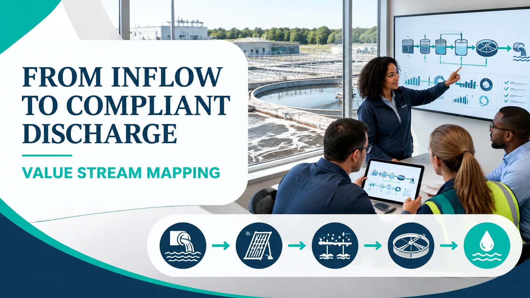
In wastewater treatment, the customer does not purchase a physical product. The value delivered is reliable treatment, compliant discharge, environmental protection, and timely operational response.
That makes Value Stream Mapping (VSM) highly relevant to utilities. The method shows how wastewater, information, alarms, samples, decisions, chemicals, energy, maintenance work and biosolids move through the system. A conventional process map may show treatment stages. A strong VSM also exposes the waiting, rework and information delays that place compliance at risk.
The Lean Enterprise Institute describes VSM as the mapping of material and information flows from start to finish. In a wastewater plant, the “material” is influent moving toward treated effluent, while information includes SCADA signals, laboratory results, alarm notifications, work orders and regulatory records.
This guide develops a worked example for a mid-size plant and shows how a future-state map can reduce alarm response lag without compromising permit controls.
1. Define the wastewater value stream and scope
The fundamental purpose of scoping is to prevent the team from attempting to improve the entire utility at once. For this example, the value stream begins when sewage enters the treatment system and ends when the plant produces compliant discharge and manages the resulting biosolids.
In scope
- Network inflow and screening
- Grit removal
- Primary clarification
- Biological nutrient removal
- Secondary clarification
- Disinfection
- Discharge and compliance sampling
- Biosolids dewatering and cartage
- Alarm generation, acknowledgement and response
- Laboratory information flow
- Maintenance response connected to process reliability
Out of scope
- Capital works delivery
- Major plant expansion
- Long-term network master planning
- Procurement of entirely new treatment facilities
The product family is one megalitre of treated wastewater released within compliance requirements. The critical-to-quality requirements include discharge compliance, stable treatment performance, traceable records, controlled energy use and dependable response to abnormal conditions.
The EPA Lean and Environment Toolkit recommends including process activity, environmental metrics, resource flows, pollution outputs and regulatory information flows in environmental VSMs. That principle is essential here: compliance information is part of the value stream, not an administrative afterthought.

2. Current-state VSM: the worked baseline
Assume the plant operates at an average inflow of 48 ML/day, with a wet-weather factor of 3.2 times average flow. During a major rainfall event, hydraulic loading can therefore approach:
48 ML/day × 3.2 = 153.6 ML/day
That swing creates a direct relationship between inflow variation and operating risk. In Lean Six Sigma terms, the process outcome can be expressed as Y = f(x): compliant discharge is influenced by critical inputs such as hydraulic load, nutrient concentration, dissolved oxygen, temperature, sludge age, chemical dose and equipment availability.
The current-state team follows both the physical flow and the information flow.
| Stage | Current-state observation | Key delay or waste |
|---|---|---|
| 1. Network inflow and screening | Influent averages 48 ML/day; wet-weather peak approaches 153.6 ML/day | Inflow shocks are detected after trends are already established |
| 2. Grit removal | Grit is removed before downstream treatment | Manual checks and reactive cleaning create avoidable interruption |
| 3. Primary clarification | Solids settle before biological treatment | Sampling and adjustment decisions rely partly on delayed results |
| 4. Biological nutrient removal | Operators adjust aeration, alkalinity and carbon dosing | 14% of operating hours are spent on corrective dosing after inflow shocks |
| 5. Secondary clarification | Biomass separation controls final suspended solids performance | Equipment faults can affect settling stability and throughput |
| 6. Disinfection | Final treatment prepares effluent for release | Chemical control depends on variable demand and manual verification |
| 7. Discharge and compliance sampling | Samples are collected, tested and recorded | 6.5 hours per day are spent on manual sampling and laboratory turnaround |
A parallel biosolids stream moves from primary and secondary solids handling to dewatering and cartage. Although it does not become compliant effluent, it consumes labour, energy, transport capacity and documentation effort. It must therefore appear on the map.
The baseline shows several critical measures:
- 31% of plant downtime is attributed to reactive maintenance.
- Average response to a process alarm is 4.8 hours.
- Discharge compliance is 91.4% during the baseline period.
- 2.3% of samples require resampling.
- Operators spend 14% of operating hours on corrective dosing adjustments after inflow shocks.
- Manual sampling and laboratory turnaround consume 6.5 hours per day.
PCE calculation
Process Cycle Efficiency (PCE) compares value-adding time with total lead time:
PCE = Value-added time ÷ Total lead time × 100
Suppose the physical treatment activities that directly transform wastewater account for 3.1 hours across a total information-and-process lead time of 29.5 hours. The baseline PCE is:
3.1 ÷ 29.5 × 100 = 10.5%
This does not imply that biological treatment or disinfection is unnecessary. It indicates that the value stream contains substantial time in waiting, sampling, decision-making, alarm escalation and rework.
3. Identify all eight DOWNTIME wastes
A wastewater VSM should identify waste in both treatment flow and information flow.
-
Defects
Non-compliant discharge, invalid sensor readings, incomplete alarm records, incorrect sample labels and laboratory results requiring resampling. -
Overproduction
Excess chemical dosing, unnecessary sludge production, duplicate alarms and samples collected more frequently than the decision requires. -
Waiting
Operators waiting for laboratory results, maintenance teams waiting for diagnostic information, and compliance staff waiting for complete records before reporting. -
Non-utilised talent
Experienced operators repeatedly correcting the same recurring alarm instead of contributing to root-cause analysis, standard work and control-plan design. -
Transportation
Physical movement of samples to the laboratory, biosolids cartage, and repeated travel between control rooms, process areas and equipment locations. -
Inventory
Work in process includes accumulated sludge, unprocessed samples, open maintenance work orders and chemical stock held to protect against uncertain demand. -
Motion
Manual meter readings, repeated rounds to confirm alarms, searching for equipment history and re-entering information across SCADA, spreadsheets and laboratory systems. -
Extra-processing
Duplicate sampling, manual transcription, repeated approval checks, separate alarm logs and laboratory confirmation that could be triggered automatically by validated exceptions.
The most urgent waste is not always the most visible. For example, a four-hour laboratory delay may appear administrative, but it can prolong dosing uncertainty and increase the risk of corrective action being applied after the process has already moved beyond its stable operating window.
4. Analyse the root causes before selecting technology
The Analyse phase of DMAIC should convert observations into evidence-based causes. The team can stratify alarm data by asset, shift, alarm class, weather condition and response owner. A Pareto chart may show that a small number of high-consequence alarms account for most response delay.
Useful analytical tools include:
- Process stratification: Compare dry-weather and wet-weather performance.
- Box plots: Examine alarm response spread by shift or process area.
- ANOVA: Test whether mean response times differ significantly across shifts or alarm categories.
- Fishbone analysis: Explore causes involving people, methods, equipment, measurement, environment and information flow.
- Measurement System Analysis: Confirm that flow meters, inline analysers and laboratory methods are sufficiently reliable. This connects with the principles in Lean 6 Sigma Hub’s guide to Measurement System Analysis.
A practical root-cause chain might be:
High wet-weather inflow → process instability → threshold alarm → alarm routed without severity classification → operator waits for confirmation → manual sample requested → laboratory result delayed → corrective dose applied late.
The opportunity is therefore broader than “install more alarms.” The improvement must address sensing, classification, response standard work, escalation and learning.
5. Design the future-state value stream
The future state should create faster information flow while preserving human judgement and regulatory governance.
Future-state design principles
- Real-time telemetry for flow, level, pH, dissolved oxygen, ammonia, turbidity and critical equipment condition.
- Inline instrumentation validated through calibration and routine verification.
- Tiered alarms: data-quality, early-warning, process-action and compliance-risk.
- Standard work specifying acknowledgement, diagnosis, action, escalation and documentation.
- Predictive maintenance using run hours, vibration, motor current, pump performance and blower efficiency.
- Automatic links between SCADA events, the maintenance management system and operator work instructions.
- Risk-based sampling rather than duplicate sampling by default.
- A single compliance dashboard that connects online data, laboratory results and required records.
- Visual management for biosolids inventory, dewatering capacity and cartage schedules.
The EPA guidance on VSM specifically supports mapping environmental data, resource use, waste streams and information sent to regulatory agencies. The future-state map should therefore make energy, chemicals, biosolids and compliance records visible alongside the wastewater flow.
| Metric | Current state | Future-state target |
|---|---|---|
| Discharge compliance | 91.4% | 98.5% |
| Average alarm response | 4.8 hours | 45 minutes |
| Resample rate | 2.3% | 0.8% |
| Energy intensity | 1,050 kWh/ML | 900 kWh/ML |
| Chemical dosing cost | $118/ML | $96/ML |
| Process Cycle Efficiency | 10.5% | 18.0% |
| Reactive-maintenance downtime | 31% of downtime | 15% of downtime |
| Corrective dosing after inflow shocks | 14% of operating hours | 6% of operating hours |
| Manual sampling and laboratory effort | 6.5 hours/day | 3.5 hours/day |
These are planning targets for the worked example, not universal regulatory benchmarks. Each plant must confirm its own permit limits, sampling obligations, safety controls and instrumentation requirements.

6. Sequence the first 90 days of kaizen
A future-state map becomes useful when translated into sequenced actions.
Days 1–30: Stabilise
- Confirm baseline definitions and data ownership.
- Classify the top 20 process alarms by consequence and frequency.
- Create standard work for alarm acknowledgement, diagnosis and escalation.
- Establish a daily tier meeting for compliance, alarms, maintenance and biosolids.
- Validate critical instruments and remove duplicate manual entries.
- Involve operations, maintenance, laboratory, compliance and IT/SCADA personnel.
Days 31–60: Pilot
- Pilot real-time telemetry for flow, ammonia, dissolved oxygen and turbidity.
- Connect selected condition indicators to predictive maintenance alerts.
- Test alarm thresholds, time delays and escalation rules on one treatment train.
- Introduce risk-based sampling triggers.
- Measure response time, resampling, energy and chemical use weekly.
- Review safety and regulatory implications before extending the pilot.
Days 61–90: Control
- Standardise successful alarm and sampling practices across the plant.
- Add control charts for compliance, response time, energy intensity and dosing cost.
- Audit standard work adherence and instrument health.
- Refresh the VSM using actual post-pilot data.
- Assign process owners and define escalation limits.
- Build the next kaizen backlog around remaining bottlenecks.

7. Build capability to sustain the gains
VSM is not a one-time drawing exercise. It is a management system for seeing the relationship between flow, variation, waste and customer requirements.
A Yellow Belt can support data collection, process observation and daily improvement. A Green Belt can lead the cross-functional project, analyse variation and validate improvements. A Black Belt can lead complex compliance and reliability projects while mentoring improvement teams.
For professionals responsible for treatment operations, process improvement, maintenance or environmental compliance, Lean 6 Sigma Hub’s CSSC-accredited Green Belt training provides practical instruction in SIPOC, data collection, hypothesis testing, root-cause analysis, piloting, SPC and control plans.
Start your Lean Six Sigma certification journey today and learn to convert wastewater process data into reliable flow, faster response and sustained compliance.
Kaizen. Kai-Care. Kai-Done. Lean Six Sigma.