Lean Six Sigma: Mean, Median, and Variance in a Bicycle Manufacturing Factory
Introduction
Lean Six Sigma combines Lean’s emphasis on eliminating waste with Six Sigma’s focus on reducing variation. This methodology helps businesses optimize processes, improve quality, and maintain consistent results.
In this article, we will analyze weekly assembly times in a bicycle manufacturing factory. Using tools like mean, median, and variance, we will calculate performance metrics, visualize process stability with a control chart, and derive actionable insights for process improvement.
Scenario: Weekly Assembly Times
The factory records the weekly assembly times (in hours) for a key production line. Below is the dataset for 12 weeks:
| Week | Assembly Time (hours) |
|---|---|
| 1 | 48 |
| 2 | 50 |
| 3 | 52 |
| 4 | 49 |
| 5 | 51 |
| 6 | 50 |
| 7 | 53 |
| 8 | 48 |
| 9 | 49 |
| 10 | 47 |
| 11 | 50 |
| 12 | 51 |
Step-by-Step Calculations
1. Mean (Average)
The mean represents the average of all data points.
Formula (Plain Text):
Mean = (Sum of all assembly times) / (Number of weeks)
Calculation (Plain Text):
Mean = (48 + 50 + 52 + 49 + 51 + 50 + 53 + 48 + 49 + 47 + 50 + 51) / 12
Mean = 598 / 12
Mean = 49.83 hours
2. Median
The median is the middle value of the data when arranged in ascending order. If there is an even number of data points, the median is the average of the two middle values.
Sorted Data (Plain Text):
47, 48, 48, 49, 49, 50, 50, 50, 51, 51, 52, 53
Middle Values:
50, 50
Calculation (Plain Text):
Median = (50 + 50) / 2
Median = 100 / 2
Median = 50 hours
3. Variance
Variance measures how far each data point is from the mean. It represents the average squared deviation.
Formula (Plain Text):
Variance = (Sum of squared deviations from the mean) / (Number of weeks)
Step-by-Step Calculation (Plain Text):
- Subtract the mean from each assembly time, then square the result:
(48 – 49.83)² = 3.34
(50 – 49.83)² = 0.03
(52 – 49.83)² = 4.69
(49 – 49.83)² = 0.69
(51 – 49.83)² = 1.36
(50 – 49.83)² = 0.03
(53 – 49.83)² = 10.12
(48 – 49.83)² = 3.34
(49 – 49.83)² = 0.69
(47 – 49.83)² = 8.00
(50 – 49.83)² = 0.03
(51 – 49.83)² = 1.36 - Add all squared deviations:
Sum of squared deviations = 3.34 + 0.03 + 4.69 + 0.69 + 1.36 + 0.03 + 10.12 + 3.34 + 0.69 + 8.00 + 0.03 + 1.36 = 33.68 - Divide by the number of weeks:
Variance = 33.68 / 12
Variance = 2.81 hours²
4. Standard Deviation
Standard deviation is the square root of the variance. It shows the extent of variation in the dataset.
Formula (Plain Text):
Standard Deviation = √Variance
Calculation (Plain Text):
Standard Deviation = √2.81
Standard Deviation = 1.68 hours
5. Control Limits for Control Chart
Control limits are calculated based on the mean and standard deviation.
Central Line (CL):
CL = Mean = 49.83 hours
Upper Control Limit (UCL):
UCL = Mean + (3 × Standard Deviation)
UCL = 49.83 + (3 × 1.68)
UCL = 49.83 + 5.04
UCL = 54.87 hours
Lower Control Limit (LCL):
LCL = Mean – (3 × Standard Deviation)
LCL = 49.83 – (3 × 1.68)
LCL = 49.83 – 5.04
LCL = 44.79 hours
Control Chart
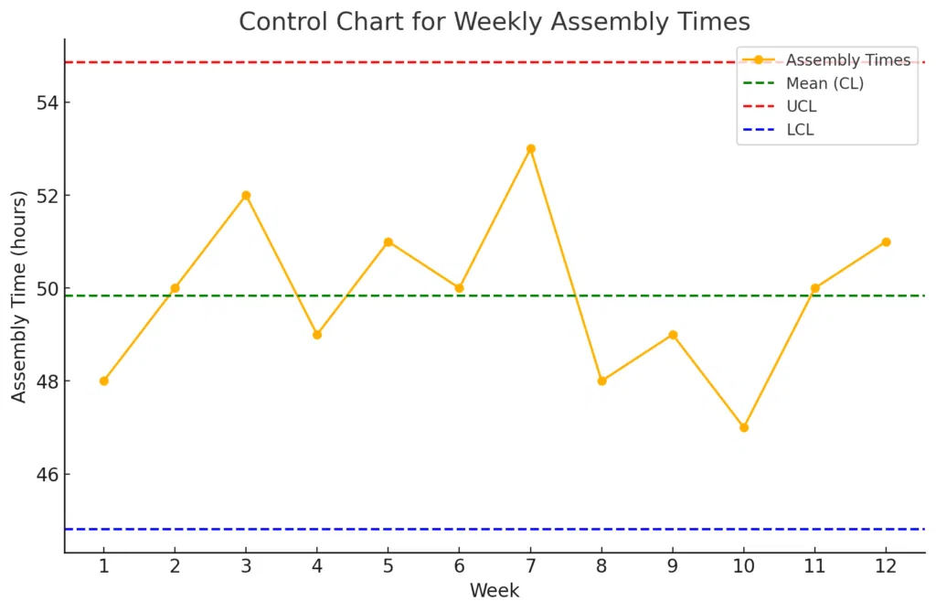
(The control chart below shows assembly times with the calculated control limits.)
Control Chart for Weekly Assembly Times

The control chart above visualizes weekly assembly times alongside the calculated control limits (UCL and LCL) and the central line (mean). This tool helps identify process stability over time.
Actionable Insights
- Monitor Process Stability:
All assembly times fall within the control limits (UCL = 54.87, LCL = 44.79), indicating a stable and consistent process. - Reduce Variation:
The standard deviation (1.68 hours) and variance (2.81 hours²) suggest minor variability. Using Lean Six Sigma tools, further standardization can optimize assembly times. - Continuous Improvement:
Implementing methods like 5S, employee training, and Kaizen events can help identify inefficiencies and improve productivity. - Regular Monitoring:
Regular updates to the control chart will ensure the process remains under control and deviations are quickly addressed.


