Hypothesis Testing Decoded: CLT, P-Values, and More Made Simple

In the realm of Lean Six Sigma, moving from the Measure phase to the Analyse phase is like transitioning from a detective gathering clues to a prosecutor building a case. Up until this point, you’ve mapped your processes and collected your data. Now, it’s time to prove what’s actually causing your defects.

To do that, we use Hypothesis Testing. For many of our students at Lean 6 Sigma Hub, this is the part of the Green or Black Belt journey where things start to feel a bit "math-heavy." But here’s the secret: you don't need to be a statistician to master this. You just need to understand the logic behind the terminology.

I’m Jvalin, and in this guide, I’m going to break down the "big four" concepts: CLT, P-values, Degrees of Freedom, and T-tests: so you can stop guessing and start proving.

The Fundamental Purpose of Hypothesis Testing

Before we dive into the jargon, let’s look at the "why." The fundamental purpose of hypothesis testing is to determine if a change in a process is real or if it’s just a result of random chance.

In any process improvement project, you will face two competing ideas:

1. The Null Hypothesis (H₀): This is the status quo. It assumes that there is no difference, no change, or no effect. It’s the "boring" option.
2. The Alternative Hypothesis (H₁): This is what you, the Six Sigma practitioner, are trying to prove. It claims that there is a significant difference or relationship.

Think of it like a courtroom. The defendant (the Null Hypothesis) is "innocent until proven guilty." You need a specific amount of evidence to "convict" the Null and accept your Alternative Hypothesis.

1. The Central Limit Theorem (CLT): The "Magic" of Statistics

If there is one concept that makes the Analyse phase possible, it is the Central Limit Theorem (CLT).

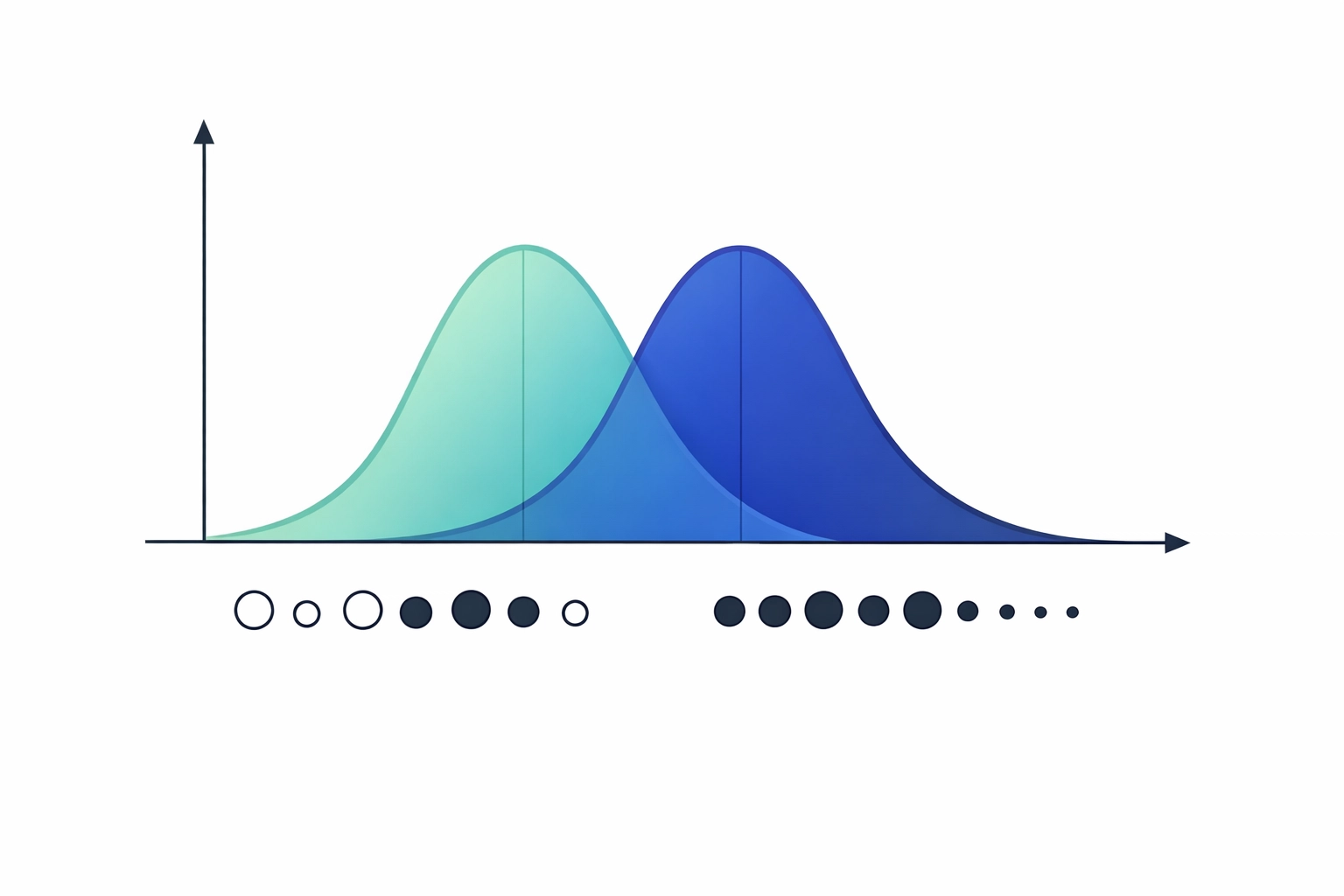
One of the biggest fears in Six Sigma is having "non-normal" data. If your data doesn't look like a perfect bell curve, you might think you can’t use standard statistical tests. The CLT is the magic that solves this.

The CLT states that regardless of the distribution of your population data, the distribution of the sample means will tend to be normal as the sample size increases (usually once you hit a sample size of 30 or more).

Why does this matter for you?
It means that even if your process data is skewed or "wonky," you can still use powerful tools like T-tests and ANOVA to find root causes. You don’t need the world to be perfect; you just need a large enough sample. This allows us to apply standardized statistical protocols to real-world, messy business data.

2. The P-Value: Your Signal-to-Noise Gauge

The P-value is perhaps the most famous (and most feared) term in statistics. Simply put, the P-value is the probability that the results you’re seeing happened by pure accident.

When you run a test in a tool like Sigma Magic, you are looking for a "threshold" for significance. In Lean Six Sigma, we typically set our "Alpha" (significance level) at 0.05.

• If P < 0.05: The result is statistically significant. You reject the Null Hypothesis. There is a "signal" in the data.
• If P > 0.05: The result is not statistically significant. You "fail to reject" the Null Hypothesis. The result is likely just "noise" or random variation.

To make it easy to remember: "If the P is low, the Null must go. If the P is high, the Null can fly."

Using the P-value allows you to make data-driven decisions. Instead of saying "I think the new machine is faster," you can say "The P-value is 0.02, meaning there is only a 2% chance this speed increase is a fluke. The machine is definitely faster."

3. Degrees of Freedom: The "Budget" for Your Data

Degrees of Freedom (df) sounds like a political concept, but in statistics, it’s about how much "freedom" your data has to vary.

To fully appreciate this, imagine you have three numbers that must add up to 10.

• You can choose any number for the first one (e.g., 5).
• You can choose any number for the second one (e.g., 2).
• But for the third number, you have no choice. It must be 3 to make the sum 10.

In this case, you had 2 degrees of freedom. In hypothesis testing, your Degrees of Freedom are usually tied to your sample size (n-1). The more data points you have, the more degrees of freedom you have, and the more "power" your test has to detect a difference. This is why having an adequate sample size is crucial in the Analyse phase.

4. T-Tests and the T-Distribution

When we want to compare the means (averages) of two groups: for example, the cycle time of Shift A vs. Shift B: we use a T-test.

The T-test relies on the T-distribution. This distribution was actually developed by a chemist at the Guinness brewery (under the pseudonym "Student") who needed a way to monitor the quality of stout with very small sample sizes.

T-Test vs. Z-Test

In a perfect world with massive datasets and a known population variance, we use a Z-test. However, in 99% of Lean Six Sigma projects, we don't know the exact population variance, and our samples aren't infinite. This is where the T-test shines.

• 1-Sample T-test: Compares a group mean against a target value (e.g., "Is our average delivery time actually 24 hours?").
• 2-Sample T-test: Compares the means of two different groups (e.g., "Is Process A faster than Process B?").
• Paired T-test: Compares the same group before and after a change (e.g., "Did the training program actually improve score results?").

Making it Easy with Sigma Magic

If reading about T-distributions and Degrees of Freedom makes your head spin, don't worry. In the modern Analyse phase, we don't expect you to do these calculations by hand with a pencil and a calculator.

Tools like Sigma Magic are designed specifically for non-statisticians. Within our CSSC-accredited training, we teach you how to plug your data into these tools. The software handles the CLT adjustments, calculates the Degrees of Freedom, and spits out a clear P-value.

Your job isn't to be a math genius; your job is to interpret the results and decide which "Vital Few" root causes are worth fixing.

A Practical Example: The Pizza Delivery Dilemma

Let’s ground this in a hypothetical case study. Imagine you are working on a project to improve delivery times for a local pizza shop.

• Current State: 35 minutes average.
• The Improvement: You implement a new GPS routing system.
• The Data: You take a sample of 40 deliveries using the new system and find an average of 32 minutes.

Is that 3-minute improvement real, or did the drivers just get lucky with traffic?

1. Hypothesis: H₀ = No change (35 mins). H₁ = Improvement (< 35 mins).
2. Test: You run a 1-Sample T-test.
3. Result: Sigma Magic tells you the P-value is 0.03.
4. Conclusion: Since 0.03 is less than 0.05, you reject the Null. The GPS system is working!

Conclusion: Data Over Guesswork

Mastering these basics: CLT, P-values, Degrees of Freedom, and T-tests: takes the guesswork out of your process improvement projects. It gives you the confidence to stand in front of leadership and say, "The data proves this is the problem."

If you’re ready to move beyond the basics and get hands-on with these tools, our Green Belt and Black Belt programs provide the templates and coaching you need to succeed.

Take the next step in your professional development and become the data-driven leader your organization needs.

Enrol in our CSSC Accredited Green Belt Program Today

Or, if you want to test your current knowledge, try our Free Lean Six Sigma Black Belt Practice Exam.