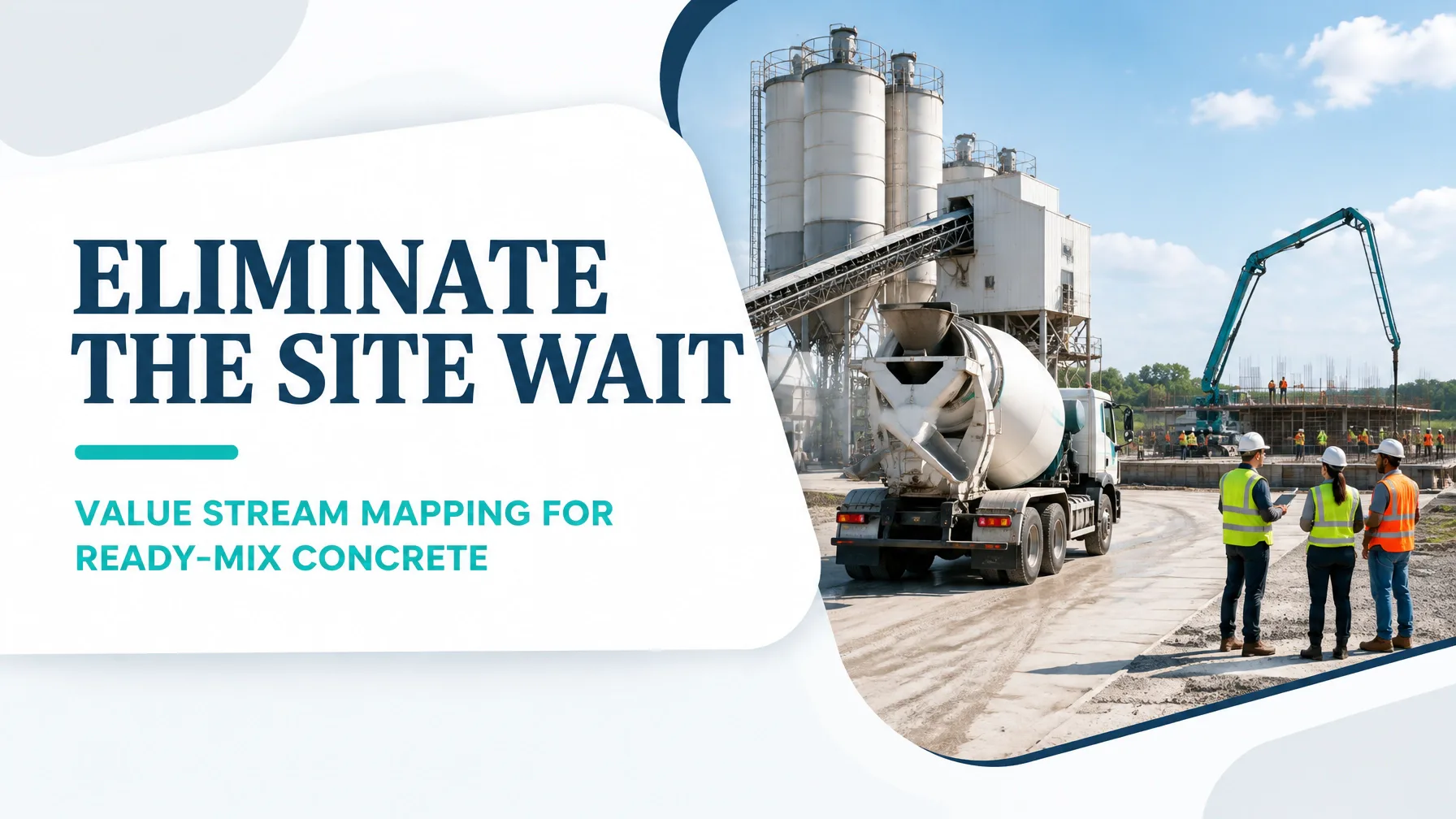
In ready-mix concrete supply, customer value is realised when the correct mix reaches the pour location on time, within specification, and ready for discharge. The concrete may be batched efficiently, yet the overall process can still lose capacity through truck queues, site access delays, slump rejections, pump interruptions and poorly sequenced washout.
Value stream mapping makes these issues visible across the complete flow. Rather than improving the batching plant, transport fleet or construction site in isolation, the method examines how material, trucks, information and decisions move from order booking to discharge complete.
This deep guide uses a worked example to show how a ready-mix supplier and construction team can map the current state, quantify the delay, identify the eight DOWNTIME wastes and design a future state with higher truck utilisation, more concrete placed per day and stronger on-time delivery.
1. Scope Selection: Define the Product Family and Boundaries
The first decision in value stream mapping is selecting a product family with sufficiently similar process steps and customer requirements.
For this example, the product family is:
Pumpable C30 structural concrete for recurring slab and footing pours, supplied in 6 m³ truckloads.
This is a practical choice because the mix design, truck capacity, quality checks, delivery requirements and discharge method are broadly consistent. Mapping one recurring family avoids combining unrelated products such as high-strength concrete, self-compacting concrete and small direct-chute orders.
Process boundaries
The map begins at:
- Order booking and pour scheduling
- Mix confirmation and dispatch planning
- Batching and truck loading
- Truck departure and travel to site
- Site arrival and queueing
- Slump testing and acceptance
- Pumping and discharge
- Washout and truck release
- Return travel to the plant
The map ends when the truck is discharge complete, washed out and released for its next assignment.
This boundary matters because the site wait is not an isolated transport problem. It is often created by the relationship between the customer’s pour rate, pump capacity, truck release pattern, dispatch decisions and washout arrangements.

2. Build the Current-State Map Step by Step
A current-state value stream map should be built from direct observation and timestamped records rather than assumptions. Capture at least 30–50 loads across comparable pours, then calculate the median and range for each activity.
Step 1: Map the information flow
Record how the order moves through the system:
- Contractor confirms the required mix, volume and pour window.
- Plant scheduler allocates batching slots and trucks.
- Dispatch sends release instructions to drivers.
- Site communicates readiness, pump availability and access conditions.
- Quality personnel record slump results and acceptance decisions.
- Dispatch reacts to delays, rejected loads or changes in pour sequence.
In many operations, the physical concrete moves faster than the information required to coordinate it. A delayed site readiness message can release several trucks into a queue before anyone has visibility of the constraint.
Step 2: Record the plant process
The example current state uses the following averages per 6 m³ load:
- Batching and mixing cycle: 8 minutes
- Truck loading: 6 minutes
- Dispatch release and ticket confirmation: 4 minutes
- Plant queue before batching or loading: 7 minutes
Although batching and loading are necessary process activities, the queue is pure delay from the customer’s perspective.
Step 3: Record transport and site activity
For the selected project:
- Plant-to-site travel: 32 minutes
- Site arrival queue: 24 minutes
- Slump testing and ticket verification: 8 minutes
- Average discharge time: 18 minutes
- Pour rate: approximately 20 m³ per hour
- Washout queue: 6 minutes
- Washout activity: 10 minutes
- Site-to-plant return: 30 minutes
The 24-minute site wait is the most visible constraint. However, the map should show the upstream and downstream effects: trucks arrive in uneven waves, the pump is intermittently starved or overloaded, and drivers spend less time available for the next load.
Step 4: Add quality and delivery data
The same 50-load sample shows:
- On-time delivery rate: 72%
- Slump-related rejection rate: 6%, or 3 loads out of 50
- Average daily volume discharged: 60 m³
- Average truck turns: 3.4 trips per truck per day
- Average end-to-end truck cycle: 142 minutes
A slump rejection does not represent only the value of the concrete. It also consumes batching time, truck capacity, driver time, transport time and site coordination effort.
Current-state flow
The physical flow can be represented as:
Order → Schedule → Batch → Load truck → Travel → Site queue → Slump test → Discharge → Washout → Return
The information flow runs in parallel:
Pour plan → Dispatch schedule → Truck release → Site readiness update → Quality acceptance → Truck release confirmation
The timeline beneath the map should distinguish processing time, necessary but non-value-adding transport, and avoidable waiting.
3. Worked Example: Quantifying the Delay
Assume a 60 m³ slab pour requiring ten 6 m³ loads.
| Current-state activity | Average time per load |
|---|---|
| Plant queue | 7 min |
| Batching and mixing | 8 min |
| Truck loading | 6 min |
| Plant dispatch confirmation | 4 min |
| Travel to site | 32 min |
| Site wait | 24 min |
| Slump test and acceptance | 8 min |
| Discharge | 18 min |
| Washout queue | 6 min |
| Washout | 10 min |
| Return travel | 30 min |
| Total cycle time | 153 min |
The operational map may report a 142-minute cycle when dispatch confirmation is embedded in another step; the important discipline is to define the timing rules consistently. In this example, the detailed timestamps expose 153 minutes from plant queue entry to truck return.
Of that total, 30 minutes is direct batching, loading, testing and discharge activity. Travel is necessary for delivery but does not transform the concrete. The remaining time is dominated by queues, coordination and vehicle movement.
For ten loads, the site requires:
- 60 m³ of concrete
- 180 minutes of discharge time at 20 m³ per hour
- A reliable truck arrival rhythm of approximately one load every 18 minutes
The current process does not consistently provide that rhythm. Trucks often arrive in clusters, wait for the pump and then return in uneven intervals.
4. The Eight DOWNTIME Wastes in Ready-Mix Supply
1. Defects
Slump-related rejections, incorrect mix tickets, over-aged concrete or contaminated loads create rework, replacement deliveries and lost capacity. The current 6% slump rejection rate is a measurable quality priority.
2. Overproduction
Releasing trucks before the pump and site crew are ready creates concrete and transport capacity ahead of actual demand. Overproduction in a perishable product increases the risk of waiting-related quality loss.
3. Waiting
The major examples are:
- Trucks waiting at the plant
- Drivers waiting at site entry
- Slump tester waiting for access
- Pump crews waiting for concrete
- Trucks waiting for washout space
The 24-minute site wait is the clearest starting point for kaizen.
4. Non-utilised talent
Drivers, dispatchers, batch operators, site supervisors and quality technicians often understand the causes of delay but are not included in daily improvement decisions. Their experience can reveal practical scheduling and layout changes that system data alone will not show.
5. Transportation
Every trip between plant and site consumes time, fuel and fleet capacity. Unnecessary repositioning, incorrect site access instructions and return trips caused by rejected or incomplete loads increase transportation waste.
6. Inventory
Work in process includes concrete in trucks awaiting discharge, trucks staged outside the site and partially completed pours waiting for the next delivery. Because concrete has a limited workable window, mobile inventory is especially time-sensitive.
7. Motion
Unnecessary driver manoeuvring, repeated ticket checks, long walks to the slump-testing point and poor washout-area layout add motion without improving the delivered product.
8. Extra-processing
Repeated phone calls, duplicate data entry, multiple ticket checks and avoidable slump retesting are forms of extra-processing. Standard digital timestamps and a single dispatch status can reduce this burden.
5. Build the Future-State Map
The future state should not simply demand that people work faster. It should redesign the flow around the customer’s required pour rhythm.
Key future-state changes include:
- Confirm site readiness through a standard pre-pour checklist.
- Release trucks using a pull signal from the site rather than a fixed sequence alone.
- Set a target arrival interval based on pump capacity.
- Establish a visible status for every truck: batching, travelling, waiting, testing, discharging, washing or returning.
- Position slump testing close to the discharge point.
- Standardise mix, ticket and adjustment procedures.
- Separate normal washout from extended cleaning requirements.
- Review the plan hourly during the pour and escalate deviations immediately.

Future-state assumptions
After the first improvement cycle, the target performance is:
- Plant queue: 3 minutes
- Batching and mixing: 7 minutes
- Truck loading: 5 minutes
- Travel to site: 30 minutes
- Site wait: 8 minutes
- Slump test and acceptance: 5 minutes
- Discharge: 15 minutes, supported by a 24 m³-per-hour pour rate
- Washout queue: 2 minutes
- Washout: 7 minutes
- Return travel: 28 minutes
- Slump rejection rate: 2%
- On-time delivery: 93%
The improved flow reduces the detailed cycle from 153 to 110 minutes, a reduction of approximately 28%. It also supports an increase from 60 m³ to 72 m³ placed per day, equivalent to moving from one standard 60 m³ pour to approximately 1.2 equivalent pours per day under comparable conditions.
Truck utilisation improves from approximately 66% to 79% when measured as the proportion of cycle time spent in planned load-bearing travel, loading and discharge activity rather than avoidable queues.
6. Current Versus Future Data Table
| Metric | Current state | Future-state target | Improvement |
|---|---|---|---|
| Average truck cycle | 153 min | 110 min | 28% reduction |
| Site wait per load | 24 min | 8 min | 67% reduction |
| Batching and loading | 14 min | 12 min | 14% reduction |
| Washout queue and activity | 16 min | 9 min | 44% reduction |
| On-time delivery | 72% | 93% | +21 percentage points |
| Slump rejection rate | 6% | 2% | 67% reduction |
| Truck turns per day | 3.4 | 4.5 | 32% increase |
| Daily discharged volume | 60 m³ | 72 m³ | 20% increase |
| Equivalent standard pours per day | 1.0 | 1.2 | 20% increase |
| Planned cycle utilisation | 66% | 79% | +13 percentage points |
These are planning targets, not universal benchmarks. Each operation should validate them against its own route distance, truck capacity, mix design, traffic conditions, pump capability, weather and project specifications.
7. Ninety-Day Kaizen Sequencing
Days 1–15: Establish the baseline
- Select the recurring product family.
- Observe at least 30 loads.
- Timestamp every process and queue.
- Measure site wait, washout delay, slump results and on-time delivery.
- Create a verified current-state value stream map.
Days 16–30: Stabilise the process
- Introduce a standard pre-pour readiness checklist.
- Define the required truck arrival interval.
- Create a single dispatch status board.
- Standardise slump sampling, acceptance and adjustment records.
- Mark the washout route and remove obvious motion waste.
Days 31–60: Run controlled experiments
- Pilot pull-based truck release on selected pours.
- Test a revised truck sequence and arrival interval.
- Trial a dedicated site contact for readiness updates.
- Compare rejection rates by travel time, weather, mix and waiting duration.
- Use a daily visual management review for missed delivery windows.
Days 61–90: Lock in the future state
- Update standard work for scheduling, dispatch, testing and washout.
- Set control limits for site wait, cycle time and slump rejection.
- Review performance weekly with plant, fleet, quality and site representatives.
- Train team members in escalation rules.
- Replicate the improved model across similar projects.
Value stream mapping is most effective when it becomes a management system rather than a one-time diagram. The future state must be monitored through practical measures that connect customer expectations to process behaviour.
Build the Capability to Improve the Whole Flow
Ready-mix concrete supply demonstrates why Lean Six Sigma must connect flow, quality, data and people. A well-designed value stream map can reveal that the largest opportunity is not a faster mixer; it may be better release timing, clearer site readiness signals, improved slump control or a washout layout that releases trucks sooner.
The Lean Six Sigma White Belt course is a practical starting point for learning core principles and DMAIC awareness. Team members supporting data collection and local kaizen can develop further through the Yellow Belt course.
Professionals leading the analysis, statistical validation and future-state implementation should consider the Green Belt certification. For complex, cross-functional supply and construction improvements, the Black Belt course develops advanced project leadership and mentoring capability.
All courses are designed for flexible, self-paced online learning and are accredited by the Council for Six Sigma Certification. Choose the belt level that matches your role, learn the method through practical case studies, and apply Lean Six Sigma to improve the flow your customers experience.
Kaizen. Kai-Care. Kai-Done. Lean Six Sigma