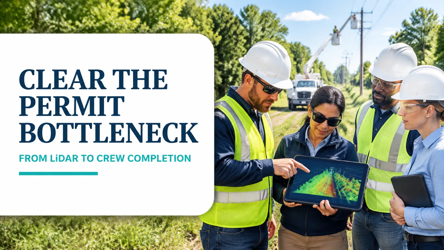
Vegetation work is often described in kilometres trimmed, spans inspected or work orders closed. Yet a utility can have capable crews and reliable LiDAR data and still miss its outage-prevention targets. The reason is frequently the flow between them: inspection findings must become prioritised work, permits and access must be resolved, and authorised tasks must reach the right crews at the right time.
Value Stream Mapping (VSM) makes that end-to-end flow visible. It maps both the information that releases work and the physical work performed in the field. For utility vegetation management, this distinction matters: a feeder segment cannot be trimmed just because a survey flags risk. It must move through decisions, approvals, scheduling, execution and verification.
The worked example below is an illustrative planning model, not a reported utility performance result. It shows how a regional utility managing 4,800 km of feeders could use VSM to find delays, establish a future state and sequence improvement work.
Set a clear value stream boundary
Map one defined flow: an aerial LiDAR survey flags a circuit segment → the crew completes the trim → the circuit is marked clear.
This endpoint matters. A completed trim is not yet reliable program evidence until quality is checked and completion is recorded. The circuit-clear status gives operations a verified view of which risk-ranked spans have been addressed and which still need action.
Permits and authorisations also need careful interpretation. Their requirements vary by jurisdiction, land rights and environmental constraints; a VSM should expose and improve the process without bypassing a required control. For example, PG&E’s transmission vegetation procedure describes project planning that considers LiDAR, land rights, environmental constraints, permits and work verification. Requirements also differ between transmission and distribution assets; refer to the applicable rules and utility standards, including FERC’s vegetation management overview.

Current state: where does the calendar go?
The table models a representative 10 km work packet. Process time (PT) is active work content; lead time (LT) is elapsed calendar time. For LiDAR, the 45-day interval is the regional flight-to-prioritised-list cycle, while the PT allocates analyst work to the packet. The fortnightly planning review is included within that 45-day interval, not added a second time.
| Current-state step | Lead time | PT | Illustrative WIP or operating detail |
|---|---|---|---|
| LiDAR flight, analysis and prioritised work list | 45 days | 1.8 days | Fortnightly review; 420 km awaiting prioritisation |
| Permit package preparation | 4 days | 0.7 days | Package and supporting records assembled |
| Regulator permit review | 28 days | 0.8 days | 310 km in permit queue |
| Contractor crew scheduling | 21 days | 0.3 days | 180 km scheduled but not started |
| Pre-work site assessment | 1.7 days | 1.7 days | 10 km ÷ 6 km/day |
| Trim execution | 4 days | 4.0 days | 10 km ÷ 2.5 km/day |
| Quality inspection | 4 days | 0.5 days | Inspection occurs four days after trim |
| GIS and work-order closeout | 3.3 days | 0.7 days | Weekly batch closeout |
| Circuit-clear confirmation | 1 day | 0.5 days | Status updated after records are complete |
| Total | 112 days | 11.0 days | Scan to verified circuit clear |
These durations sum to 112 days. The flow’s largest single delay is the 28-day permit review, followed by the 21-day contractor scheduling queue. The permit queue is the bottleneck to address first, not by weakening the approval standard, but by improving when and how complete work enters review.
The takt calculation provides a separate capacity check. If the utility needs 1,200 km cleared each year and has 120 effective field-working days in its planned vegetation work window, takt is 1,200 ÷ 120 = 10 km per working day. The current illustrative output of 900 km/year, or 7.5 km per effective day, falls short.
Current process time is 11 days. For the PCE calculation, assume 6 days of that time are value-adding work on the defined packet; the remainder is avoidable or administrative touch effort. Current PCE is therefore 6 ÷ 112 = 5.4%. Confirm this classification with teams before using the measure: PCE depends on a consistent definition of value-adding time.
Locate the DOWNTIME wastes in the real workflow
Use the eight wastes as a diagnostic, not a reason to rush safety, environmental review or quality checks.
- Waiting: segments sit between permit approval and crew availability.
- Defects: missed clearance specifications trigger re-inspection and rework.
- Inventory: a backlog of work accumulates while awaiting permits.
- Transportation: crews travel between non-contiguous segments.
- Motion: field teams walk lines again to re-flag spans already identified in the data.
- Overprocessing: teams repeat LiDAR analysis on circuits trimmed since the previous survey.
- Non-utilised talent: arborist findings do not make it into crew briefings.
- Overproduction: lower-risk segments are trimmed ahead of higher-risk spans.
A real utility example illustrates why better information can support program decisions. DTE Energy’s high-density distribution LiDAR project reported a projected return of 10.5 times its initial investment in data-gathering technology. That figure belongs to DTE’s case and should not be treated as a forecast for another utility; the transferable lesson is to connect data, prioritisation and work execution.
Future state: release work earlier, then level crew flow

A practical future state changes the sequence and information handoffs:
- Submit permits on a rolling basis while LiDAR analysis continues. Prepare applications as soon as candidate spans and required records are available, rather than waiting for a complete regional list.
- Sequence work by risk. Release the highest-risk spans first, subject to applicable approvals, access and operating constraints.
- Level crew scheduling to takt. Plan authorised work toward the required 10 km per effective working day, using crew capacity and local conditions rather than allowing a large batch queue to build.
- Build contractor pre-brief packs from arborist data. Include span locations, prescribed work, access notes and relevant constraints so crews can prepare without re-flagging information already available.
- Combine trim closeout with same-day QA where practical. Record results promptly and direct any missed-clearance items into a defined correction loop.
- Replace weekly GIS batching with daily electronic completion. Update work orders and circuit-clear status when verified records are ready.
In the illustrative future-state model, these changes reduce scan-to-clear lead time to 61 days and active process time to 4.6 days. Assuming the future 4.6 days are value-adding for this packet, PCE becomes 4.6 ÷ 61 = 7.5%. These are planning targets for testing, not guaranteed outcomes.
| Measure | Current state | Future-state target |
|---|---|---|
| Scan-to-clear lead time | 112 days | 61 days |
| Active process time (PT) | 11.0 days | 4.6 days |
| Process cycle efficiency (PCE) | 5.4% | 7.5% |
| Permit-queue WIP | 310 km | 90 km |
| Crew scheduling WIP | 180 km | 60 km |
| Cleared per effective day vs takt | 7.5 km/day vs 10 | 10 km/day vs 10 |
| Trim-miss rework rate | 12% | 4% |
The target rework rates, WIP and output figures are scenario assumptions for this worked example. Establish actual baselines from work-order, permit, inspection and GIS records, then review the measures together. In particular, confirm that faster flow is not achieved at the expense of clearance quality, compliance or safe field execution.
Sequence a 90-day kaizen
Days 1–30: Parallel permitting and risk-ranked sequencing
- Agree risk-ranking rules with vegetation, grid operations, environmental and regulatory stakeholders.
- Pilot rolling permit submissions on a defined feeder group.
- Track application completeness, permit cycle time and kilometres in the permit queue.
Days 31–60: Crew levelling and pre-brief packs
- Plan authorised work toward the 10 km-per-effective-day takt.
- Test contractor briefs built from arborist and LiDAR information.
- Monitor crew utilisation, travel between segments and trim-miss rework.
Days 61–90: Daily closeout and QA merge
- Trial same-day QA and trim closeout where operationally appropriate.
- Replace weekly closeout batches with daily electronic updates.
- Review lead time, PCE, verified kilometres cleared and compliance exceptions; standardise only after results are confirmed.

Build the capability to improve the whole system
A VSM is most useful when teams can distinguish evidence from assumptions, measure a baseline and test changes through structured problem-solving. Lean Six Sigma training develops those skills: from process mapping and data collection to root-cause analysis, piloting and control.
Explore Lean Six Sigma training from White Belt to Master Black Belt at Lean 6 Sigma Hub. Courses are CSSC-accredited and self-paced online, with practical learning through real DMAIC case studies, simulations, dummy data, charts and worked examples. The Green Belt course is one pathway for professionals who want to lead data-driven improvement projects.
Choose a Lean Six Sigma certification pathway and build the capability to turn process data into safer, more reliable flow.
Kaizen. Kai-Care. Kai-Done. Lean Six Sigma.