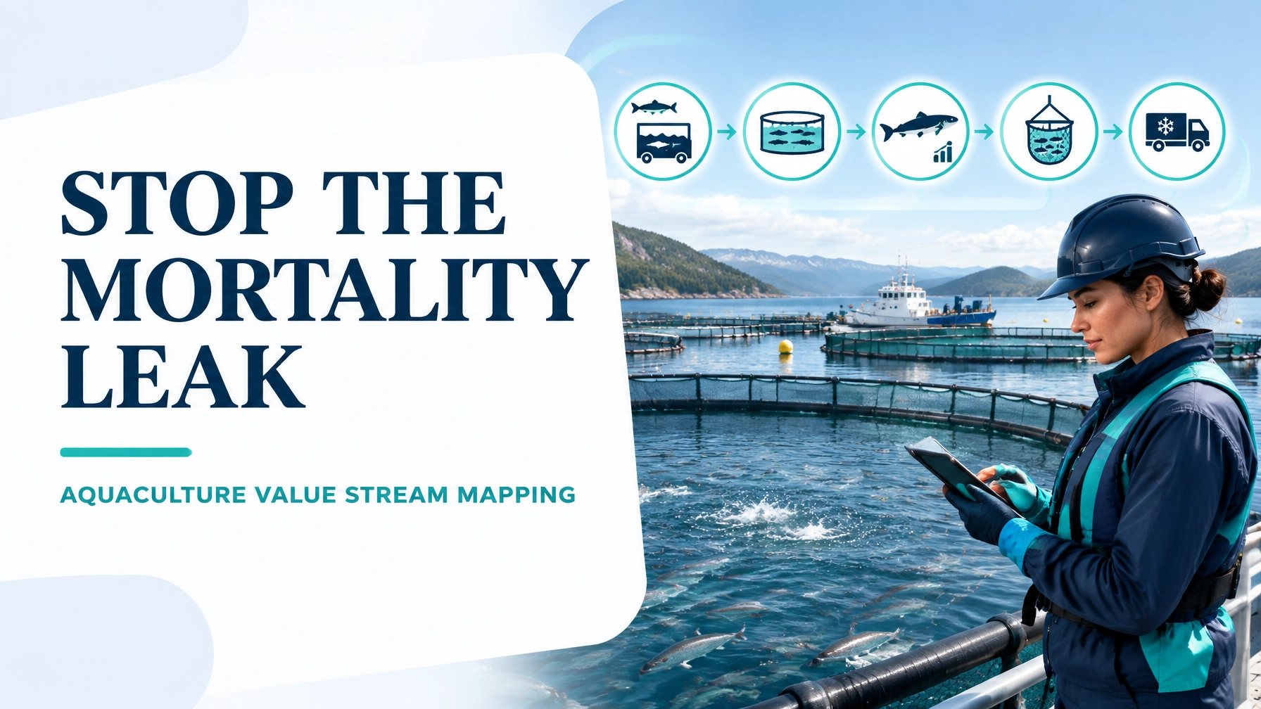
In aquaculture, a one-percentage-point mortality increase can represent thousands of dollars in lost product, additional feed consumed per kilogram harvested, and reduced production capacity. Yet mortality is rarely caused by one isolated event. It emerges across a value stream: smolt transfer, feeding, water-quality variation, disease control, sea lice treatments, grading, harvest scheduling, processing, and cold-chain dispatch.
Value Stream Mapping (VSM) makes that entire system visible. It connects fish counts, biomass, information flow, handling time, waiting, treatment events, yield and customer requirements in one operational picture.
This guide uses a worked salmon-style marine cage example. The numbers are illustrative but grounded in reported industry benchmarks. Commercial salmon operations commonly report 80–90% whole-cycle survival, FCR of approximately 1.1–1.4, harvest weights near 4–5 kg, sea grow-out periods of 14–24 months, and edible yields around 73–74%. See the Salmon Industry Handbook and recent aquaculture research for wider context.
The Aquaculture Value Stream: What Must Be Mapped?
The fundamental purpose of VSM is to show how value, material and information move from supplier to customer. For a finfish farm, the value stream begins with juvenile fish and ends with chilled product delivered to a processor, retailer, food-service customer or distributor.
Map these connected stages:
- Smolt or juvenile transfer into grow-out.
- Feeding and biomass growth.
- Water-quality and environmental monitoring.
- Fish-health checks and mortality recording.
- Sea lice monitoring and treatment.
- Grading, handling and cage management.
- Harvest planning and scheduling.
- Harvesting, slaughter and chilling.
- Primary or secondary processing.
- Cold-chain dispatch and customer delivery.
The map must include both fish flow and information flow. A lice count, dissolved-oxygen alert or harvest forecast can change the physical flow of fish within hours.

Worked Example: Quantifying the Mortality Leak
Assume a farm stocks 100,000 smolts into marine cages.
| Measure | Current-state assumption |
|---|---|
| Smolts stocked | 100,000 |
| Transfer mortality | 2.0% |
| Fish entering grow-out | 98,000 |
| Sea-phase survival | 85.0% |
| Fish harvested | 83,300 |
| Average harvest weight | 4.5 kg |
| Harvested live biomass | 374,850 kg |
| Sea grow-out period | 15 months |
| Feed conversion ratio | 1.30 |
| Sea lice treatment cycles | 4 |
| Handling days per treatment | 2 |
| Edible processing yield | 73.5% |
The resulting edible product is:
374,850 kg × 73.5% = 275,515 kg
If the operation sells finished product at an assumed $8 per kg, the revenue represented by the harvest is approximately $2.20 million, before processing, logistics and operating costs.
Now consider one additional mortality percentage point, calculated against the original 100,000 smolts:
- 1,000 fish lost
- 1,000 × 4.5 kg = 4,500 kg live biomass
- 4,500 × 73.5% = 3,308 kg edible product
- 3,308 × $8 = $26,460 of product value
This is the value represented by a one-percentage-point reduction in survival under this scenario. The calculation excludes avoided feed, treatment, handling and processing costs, so the economic impact may be greater.
Current-State VSM: Find the Constraint, Not Just the Symptom
A current-state map should show process time, waiting time, inventory or work in process, batch sizes, decision points and quality losses.
| Process step | Key data | Time or delay | Primary risk |
|---|---|---|---|
| Smolt transfer | 100,000 fish; 2% transfer mortality | 2 days | Handling and salinity stress |
| Grow-out and feeding | FCR 1.30; 15 months | 450 days | Feed waste, disease, variation |
| Monitoring | Daily biomass, oxygen, temperature and lice checks | Continuous | Delayed escalation |
| Lice treatments | 4 cycles × 2 handling days | 8 handling days | Treatment stress and mortality |
| Harvest scheduling | Weekly customer demand | 7-day average wait | Fish held beyond optimum size |
| Harvest and chilling | 4.5 kg average fish | 1–2 days | Capacity and welfare risk |
| Processing | 73.5% edible yield | 1 day | Trim, grading and yield loss |
| Cold-chain dispatch | Chilled product | 1–2 days | Temperature excursions |
The total biological cycle cannot be compressed like a factory assembly line. However, VSM distinguishes necessary growth time from avoidable waiting, repeated handling, information delay and rework.
For example, research has associated non-medicinal sea lice treatments with substantially increased monthly mortality. Therefore, the question is not simply, “How many treatments occurred?” It is:
- What triggered each treatment?
- How quickly was the trigger detected?
- Was the treatment effective?
- How many days of feeding and growth were disrupted?
- What mortality occurred during the following seven and thirty days?
- Did treatment outcomes vary by cage, vessel, crew or water temperature?
Analyse Phase: Trace Mortality to Root Cause
During the Analyse Phase of DMAIC, the team separates correlation from root cause using evidence rather than assumptions.
Start by stratifying mortality by:
- Cage and site.
- Week after smolt transfer.
- Water temperature and dissolved oxygen.
- Feed quantity and feeding response.
- Treatment type and treatment crew.
- Fish size and grading history.
- Disease status and handling duration.
Useful tools include Pareto charts, cause-and-effect diagrams, run charts, control charts, box plots and hypothesis tests. A box plot may reveal that one cage has a wider mortality distribution than the others. ANOVA can compare mean mortality across three or more cages, sites or treatment methods. Bartlett’s Test can assess whether group variances are sufficiently equal before applying ANOVA. Always validate the measurement system first: inconsistent fish counts, delayed carcass collection or biased sampling can make a stable process appear unstable.
The output should be a verified relationship such as:
Fish exposed to treatment handling longer than 90 minutes had a 1.8-times higher seven-day mortality rate than fish handled within 60 minutes, after stratifying by cage and temperature.
That is more actionable than stating that “treatments cause losses.”
Future-State Design: Protect Flow and Fish Welfare
A practical future-state design could target:
- Transfer mortality reduced from 2.0% to 1.0%.
- Sea-phase survival improved from 85.0% to 88.0%.
- Treatment cycles reduced from four to three, through earlier monitoring and coordinated action.
- Average treatment handling reduced from two days to one day.
- Harvest scheduling wait reduced from seven days to two days.
- Processing yield improved from 73.5% to 74.5%.
- Dispatch temperature compliance increased to 100% of documented loads.
The revised flow is not based on a single intervention. It is sequenced through Kaizen:
- Stabilise measurement: standardise fish counts, mortality definitions, biomass estimates, feed records and temperature sensors.
- Reduce response delay: create clear lice and water-quality escalation thresholds.
- Improve treatment preparation: use standard work, pre-checks, equipment readiness and handling-time targets.
- Control bottlenecks: align harvest capacity, processing slots, vessels, transport and customer demand.
- Improve yield: measure weight at harvest, gutting, filleting, trimming and packing.
- Control the gains: use weekly survival, FCR, treatment mortality, yield and cold-chain dashboards.

The Lean Six Sigma Concepts Behind the Map
- Value: customer willingness to pay defines which activities matter.
- Value Stream: all material and information steps from smolt to delivered product.
- Value Stream Mapping: current- and future-state maps reveal waste and leverage points.
- Waste (Muda): the eight DOWNTIME wastes include defects, overproduction, waiting, non-utilised talent, transportation, inventory, motion and extra-processing.
- Waiting: idle vessels, crews, materials, information or harvest slots signal poor flow.
- Work in Process: fish in cages, harvested fish awaiting processing and packed product awaiting dispatch are forms of WIP.
- Bottleneck: a constrained treatment vessel, harvest crew, processor or cold store limits total throughput.
- Takt Time: available processing time divided by customer demand sets the required dispatch rhythm.
- Throughput: harvested or dispatched kilograms per week indicate process capacity.
- Theory of Constraints: improve the limiting factor first, then re-evaluate the system.
- Variation: common-cause and special-cause fluctuations require different corrective actions.
- Voice of the Customer: freshness, size, delivery window and traceability become measurable CTQs.
- Voice of the Business: margin, biomass utilisation, compliance and capacity must balance customer needs.
- Voice of the Process: actual data shows whether the stream meets those requirements.
- Y = f(x): harvest yield, survival and quality are outcomes influenced by critical inputs such as oxygen, feed, temperature and handling time.
- Attribute Data: Pass/Fail cold-chain checks, treatment completed/not completed and mortality cause categories support quality analysis.
- Average (Mean): mean harvest weight, FCR and weekly mortality establish performance baselines.
- Z-Score: standard deviations from the mean help compare cage or site performance.
- X-bar Chart: monitoring average biomass or process weight with an R chart can reveal shifts and trends.
- Andon: visual alerts can signal low oxygen, abnormal feeding, rising lice counts or temperature excursions in real time.
- Autonomation (Jidoka): intelligent monitoring can detect abnormal conditions and trigger a controlled response.
- Affinity Diagram: large volumes of crew observations can be grouped into natural themes such as equipment, training, biology and scheduling.
- Agile: short, iterative improvement cycles complement DMAIC pilots when environmental conditions change.
- Approval: formal health, harvest and compliance checkpoints support governance but can create bottlenecks.
- Break-Even Analysis: compares treatment, monitoring or automation cost with the value of recovered biomass and yield.
- Business Case: quantifies survival, FCR, yield, capacity and customer benefits to secure leadership support.
- Zero Defects: Crosby’s principle of doing things right the first time translates into accurate counts, correct handling and compliant temperature control.
- White Belt: introduces basic Lean Six Sigma principles and DMAIC awareness.
- Yellow Belt: supports data collection, standard work and larger improvement projects.
- Black Belt: leads advanced projects, statistical analysis and Green Belt mentoring.
- Time Observation Sheet: records actual handling, transfer, harvest and processing times to separate value-added work from delay.
- Approval, data quality and governance should be designed into the VSM rather than added after problems occur.

Build Capability to Improve the Whole Stream
A mortality leak is rarely solved by asking operators to work faster. It is solved by connecting biological performance, process discipline, statistical analysis and customer demand.
A trained improvement team can create a living VSM that is updated by cage, cohort, treatment event and harvest week. Lean 6 Sigma Hub’s online training develops these skills through self-paced learning, practical case studies and applied tools. Professionals leading aquaculture improvement work may also consider the CSSC-accredited Green Belt programme to strengthen project leadership, data analysis and control planning.
Map the stream, quantify every loss, and pursue Lean Six Sigma certification to lead measurable aquaculture improvement.
Sources and further reading
- Mowi Salmon Industry Handbook
- Frontiers in Aquaculture: salmon welfare and production research
- GAIN Report on Value Chain Mapping
- Nordic salmon processing yield report
Kaizen. Kai-Care. Kai-Done. ( Lean Six Sigma)