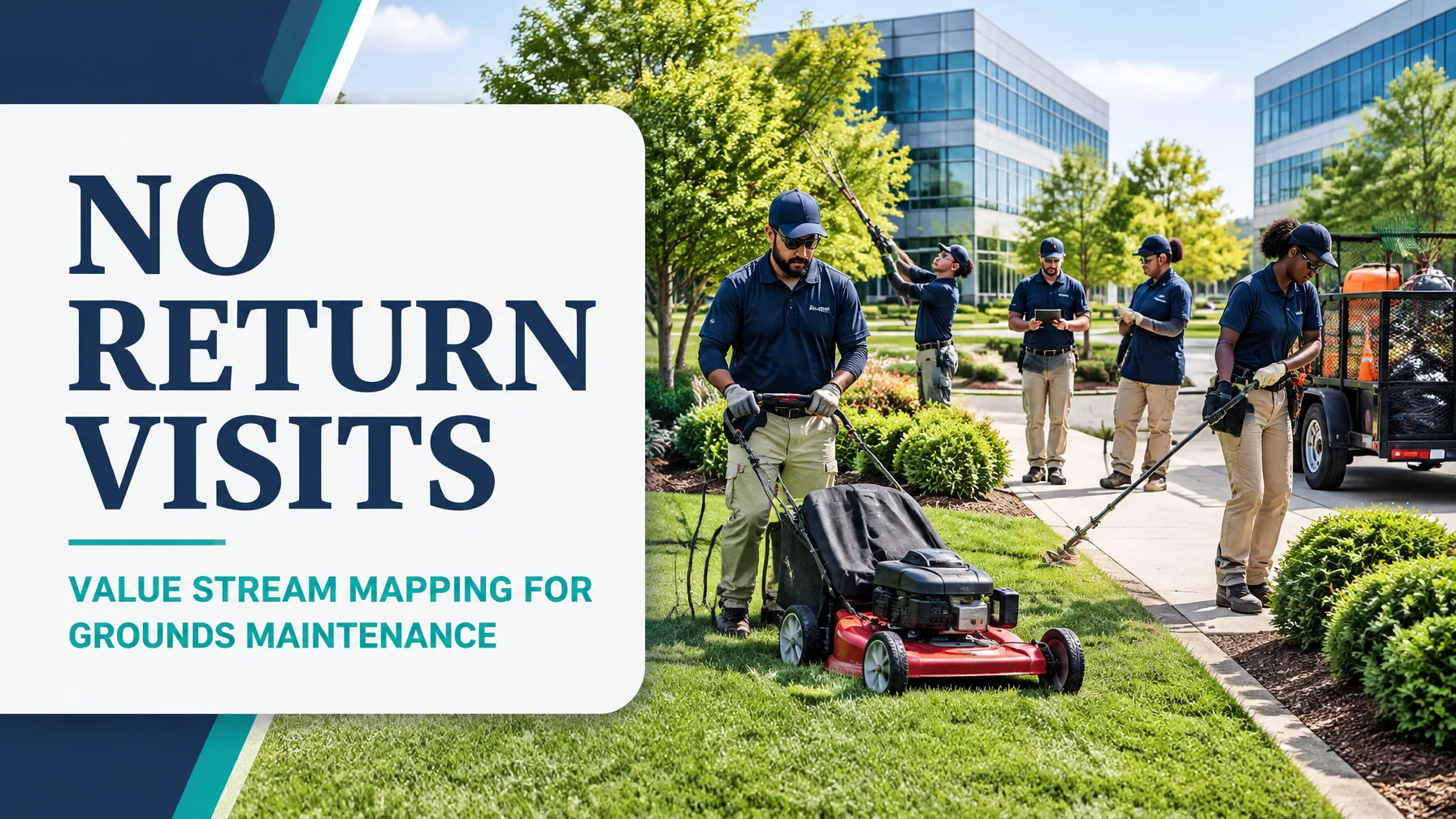
In commercial landscaping and grounds maintenance, the value stream is not a single job. It is a repeating service cycle: work order, route planning, mobilisation, site execution, inspection, sign-off and invoicing, then the cycle begins again.
For the property or facilities manager, value is straightforward: presentable, safe, defect-free grounds at the agreed standard, every visit. They do not primarily value internal scheduling effort, duplicated paperwork or a crew returning because the correct equipment was unavailable.
This makes grounds maintenance a flow problem rather than simply a labour problem. Seasonal demand changes the workload, while route design determines how much of each paid day is spent producing visible value versus travelling, waiting, searching or correcting defects.
Value Stream Mapping (VSM) makes that entire service system visible. It connects the physical flow of people, equipment and green waste with the information flow of work orders, variations, run sheets, photographs and approvals.
1. Scope Selection: Define the Maintenance Product Family
The selected product family is a 45-site commercial portfolio serviced on a four-week cycle.
The map begins at:
- Contract award or work-order release.
- Pre-start site mobilisation and route planning.
- Scheduled visit execution: mowing, edging, pruning, spraying and litter removal.
- Green-waste removal.
- Quality inspection.
- Client sign-off.
- Invoicing.
The map excludes construction landscaping projects and one-off tree works, because those services have different resource profiles, approval gates and process routes.
This boundary is essential. A VSM becomes difficult to act on when recurring maintenance, capital works and emergency call-outs are blended into one family. A clearly defined scope supports a stronger project scope boundary, more reliable data and a more useful future state.
2. Current-State Mapping: Where Flow Breaks Down
The current state should be built by observing actual routes, not by relying only on office assumptions. A cross-functional team should include the operations manager, scheduler, area supervisor, crew lead, quality inspector and invoicing administrator.

Current-state process boxes
| Process box | Cycle time or workload | Crew/resource | Travel | Uptime / first-time-right | Queue or information issue |
|---|---|---|---|---|---|
| Work-order release and triage | 2.0 days average | 1 scheduler | 0 hours | 92% information completeness | 18 open work orders |
| Route planning and dispatch | 6 scheduler-hours per cycle | Scheduler plus area supervisor | 0 hours | 84% schedule stability | Email variation requests |
| Pre-start mobilisation | 4 crew-hours per route | Crew lead plus crew | 0 hours | 63% kit-complete readiness | Paper run sheets and missing equipment |
| Site execution | 1,180 scheduled crew-hours per cycle | Field crews | 268 hours between sites | 81% first-time-right | Phone calls from tenants |
| Rework and return visits | 94 crew-hours per cycle | Field crews and supervisor | Included in route burden | 19% of visits not first-time-right | Defect loop after inspection |
| Quality walk and sign-off | 12% of sites fail the walk | Area supervisor or client | Additional site travel where required | 88% pass rate | Photos and notes stored inconsistently |
| Invoice preparation | 2–6 days after completion | Administration | 0 hours | 78% complete documentation | Delayed approvals and missing evidence |
The physical flow is interrupted by missing tools, uneven route density and defects discovered only after the crew has left. The information flow is equally important: email variation requests, paper run sheets and phone calls from tenants create multiple versions of the truth.
3. Worked Example: Four-Week Portfolio Cycle
The portfolio contains 45 sites, with 1,180 scheduled crew-hours per four-week cycle.
Total lead time
The average work-order-to-invoice lead time is:
22 days × 24 hours = 528 elapsed clock-hours
That is the customer-facing lead time. However, because several crews work in parallel, the 528 clock-hours cannot be directly divided into aggregate crew-hours without distorting PCE.
For the work-content view, calculate total crew-hours consumed:
- Scheduled on-tool work: 1,180 hours
- Travel between sites: 268 hours
- Rework and return visits: 94 hours
Total work-content time = 1,180 + 268 + 94 = 1,542 crew-hours
Value-added time on the tools
The 94 rework hours do not create new customer value. They correct work that should have been completed during the original visit.
Value-added time = 1,180 − 94 = 1,086 crew-hours
Process Cycle Efficiency
Using the work-content definition:
PCE = Value-added time ÷ Total work-content time × 100
PCE = 1,086 ÷ 1,542 × 100 = 70.4%
Therefore, approximately 29.6% of the measured crew-hour content is travel or rework. The 22-day external lead time remains the critical customer metric, while the 70.4% PCE reveals how much field effort is not directly delivering the agreed grounds standard.
Crew utilisation
Assume the portfolio is supported by 12 crews, each with 40 available hours per week, across four weeks:
Available capacity = 12 × 40 × 4 = 1,920 crew-hours
Productive scheduled utilisation:
1,180 ÷ 1,920 × 100 = 61.5%
Total field deployment, including scheduled work, travel and rework:
1,542 ÷ 1,920 × 100 = 80.3%
The gap between 61.5% productive utilisation and 80.3% deployed capacity is a strong signal that route design and first-time-right performance are consuming capacity.
Route density
Average productive work per site:
1,180 ÷ 45 = 26.2 crew-hours per site
Travel burden per site:
268 ÷ 45 = 5.96 travel hours per site
Route density ratio:
1,180 ÷ 268 = 4.40 productive crew-hours for every travel hour
This is not a universal benchmark; it is the baseline for this portfolio. Its purpose is to show where geographic clustering and zone-based scheduling can release capacity.
4. The Eight DOWNTIME Wastes in the Field
Using a fully loaded labour assumption of $55 per crew-hour and 13 four-week cycles per year, the following estimates show the economic importance of the waste categories. They are directional and should be validated during the Measure phase.
- Defects: The 94 rework hours per cycle equal 1,222 annual hours, or approximately $67,210. Example: a bed edge is missed and the crew returns after a quality complaint.
- Overproduction: Unplanned mowing or duplicate visits consume an estimated 20 hours per cycle: 260 annual hours, or $14,300.
- Waiting: Access delays, unclear variations and approval holds consume an estimated 80 hours per cycle: 1,040 annual hours, or $57,200.
- Non-utilised talent: Supervisors spend an estimated 24 hours per cycle manually reconciling notes instead of coaching crews or improving standards: 312 annual hours, or $17,160.
- Transportation: If only 30% of the 268 travel hours is avoidable, the opportunity is 80.4 hours per cycle: approximately 1,045 annual hours, or $57,475.
- Inventory: Excess, misplaced or expired consumables create an estimated $9,000 annually in carrying, emergency purchase and disposal costs.
- Motion: Searching for keys, tools, attachments and site instructions consumes an estimated 42 hours per cycle: 546 annual hours, or $30,030.
- Extra-processing: Duplicate entry from paper run sheets into office systems consumes an estimated 36 hours per cycle: 468 annual hours, or $25,740.
These figures should not be added automatically because some categories overlap. They are a prioritisation tool for the Cost of Poor Quality calculator.
5. Future-State Build: Design Flow Around Customer Demand
The future state should reduce variation at the source rather than depend on final inspection to find every problem.

The redesigned flow includes:
- Geographic route levelling: Divide the portfolio into practical zones and schedule nearby sites together.
- Zone-based scheduling: The four-week demand is 45 visits, or 11.25 site visits per week. A five-day operating week therefore requires approximately 2.25 site visits per day across the portfolio, adjusted for site size and crew-hours.
- Standard work by site type: Create repeatable standards for office parks, retail centres, industrial estates and mixed-use properties.
- Photo-verified standards: Define acceptable mowing height, edging finish, litter-free areas, pruning limits and bed presentation through reference photographs.
- Kit-of-parts trailer loadout: Standardise trailer contents by service type, including mowing, pruning, spraying and waste removal kits.
- First-visit-right checklists: Confirm access, equipment, PPE, chemicals, waste capacity, variation instructions and site-specific risks before dispatch.
- Mobile digital run sheets: Replace paper records with a single work order containing tasks, customer requirements, photographs and exceptions.
- Photo sign-off: Require before-and-after evidence for defined critical-to-quality points.
- Two-bin consumable replenishment: Use a visual trigger for line trimmer cord, fuel, bags, spray materials and PPE.
- Seasonal demand levelling: Pre-agree optional works, such as mulch, seasonal pruning or storm preparation, so peak demand is planned rather than inserted into routes at short notice.
- Visual weekly completion board: Display assigned, in-progress, complete, inspection-passed and exception work by zone.
6. Current State vs Future State
The following future-state figures are improvement targets for the worked example, not universal industry benchmarks.
| Metric | Current state | Future-state target |
|---|---|---|
| Cycle lead time | 22 days | 14 days |
| Value-added crew-hours | 1,086 | 1,120 |
| Process Cycle Efficiency | 70.4% | 86.8% |
| Travel as a share of field work | 18.5% | 11.8% |
| First-time-right | 81% | 90% |
| Return visits per 100 visits | 19 | 8 |
| Work-order-to-invoice time | 22 days | 14 days |
| Productive crew utilisation | 61.5% | 70% |
| Client quality score | 88/100 | 95/100 |
The future-state PCE assumes approximately 1,120 value-added hours, 150 travel hours and 20 rework hours:
1,120 ÷ (1,120 + 150 + 20) × 100 = 86.8%
7. 90-Day Kaizen Sequencing
Days 1–30: Stabilise and measure
- Operations manager: Confirm scope, baseline lead time, PCE, FTR and client quality score.
- Area supervisor: Observe representative routes and record travel, waiting, defects and failed quality walks.
- Crew lead: Build site-type checklists and photograph current standards.
- Metric that moves: Data completeness, baseline accuracy and equipment-readiness rate.
Days 31–60: Pilot the future state
- Operations manager: Create geographic zones and level the four-week schedule to demand.
- Area supervisor: Pilot mobile run sheets, photo sign-off and weekly visual completion boards.
- Crew lead: Test kit-of-parts trailer loadouts and first-visit-right checks.
- Metric that moves: Travel hours, first-time-right percentage and return visits per 100 visits.
Days 61–90: Lock in and expand
- Operations manager: Approve standard work and integrate optional seasonal works into contracts.
- Area supervisor: Audit adherence, coach exceptions and review quality trends weekly.
- Crew lead: Operate two-bin replenishment and update standards when recurring causes appear.
- Metric that moves: Work-order-to-invoice time, PCE, productive crew utilisation and client quality score.
8. Build the Capability to Improve the Value Stream
This example uses practical Lean Six Sigma tools: current-state mapping, future-state mapping, takt, standard work and Process Cycle Efficiency. It also combines operational observation with numerical analysis, which is essential when the objective is reliable service rather than a visually attractive map.
To develop these skills systematically, explore Lean Six Sigma concepts and glossary resources, then pursue CSSC-accredited Green Belt or Black Belt training at Lean 6 Sigma Hub. Green Belt training is suited to professionals leading focused improvement projects; Black Belt training develops the capability to lead complex change, analyse variation and mentor improvement teams.
Build the capability to map your service value stream, calculate its performance and lead the future state through CSSC-accredited Lean Six Sigma Green Belt or Black Belt training at lean6sigmahub.com.
Kaizen. Kai-Care. Kai-Done. Lean Six Sigma