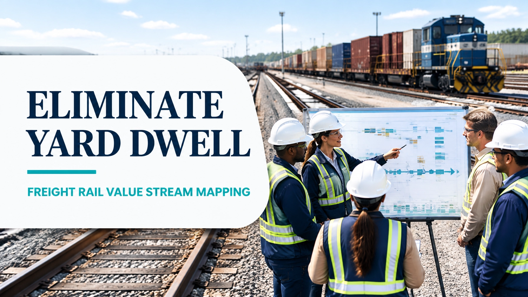
In freight rail, network velocity is determined by more than line-haul speed. A railcar can travel hundreds of kilometres efficiently and still deliver poor customer performance if it spends excessive time waiting in a yard.
For carload operations, yard dwell is often the dominant component of transit time. Research on classification terminals has found that approximately 59% to 64% of railcar transit time can be spent in yards. The operational consequence is significant: longer dwell reduces car velocity, increases equipment requirements, disrupts train connections and raises exposure to avoidable cost.
Value Stream Mapping (VSM) provides a disciplined way to see the complete flow of material and information. Rather than focusing only on the hump, a freight rail VSM connects the customer’s consignment request, car availability, documentation, switching, classification, crew calls and loading-track placement in one system view.
This guide presents a worked freight rail example using Lean Six Sigma, Theory of Constraints and practical kaizen sequencing.
1. Select the Right Freight Rail Scope
A VSM is only useful when its boundaries are precise. For this case, the scope is:
Customer consignment request → car order and release → origin yard receipt → inspection → classification → staging → loaded railcar placed at the origin loading track.
The map excludes:
- Long-haul line haul
- Intermediate classification yards
- Destination delivery
- Customer unloading and empty-car release
However, one downstream metric remains visible: release-to-departure time. This prevents the team from improving origin placement while simply transferring delay to the next operating stage.
The fundamental purpose is to understand how quickly a customer request becomes a usable, correctly positioned railcar: and where waiting, rework and unnecessary movement consume the available capacity.

2. Current-State Freight Rail VSM
Consider a representative origin yard handling 1,150 carloads per month, or approximately 38 carloads per day across a 30-day operating month.
The baseline data is:
| Measure | Current state |
|---|---|
| Monthly carloads | 1,150 |
| Average yard dwell | 34 hours |
| Target yard dwell | 18 hours |
| Hump processing rate | 12 cars/hour |
| Average release-to-departure time | 9.5 hours |
| Crew availability gap | 6.0 hours per affected car |
| Departure reliability | 72% |
| Demurrage-related cost exposure | $145/car |
| Switcher fuel consumption | 18 gallons/car |
Current-state flow
-
Consignment request received
The customer requests a car, commodity movement and loading window. Missing specifications or late changes create information delays. -
Car order and equipment assignment
The planning team searches for available equipment. Cars may remain in a standing-car pool because the order is not synchronised with the loading schedule. -
Car release and origin receipt
A released car enters the yard, but receipt confirmation, inspection and documentation may occur in separate systems. -
Inspection and exception handling
Defects, bad-order conditions or incomplete documentation can divert cars to repair or holding tracks. -
Hump classification
The hump processes cars at an average rate of 12 cars per hour. This figure looks productive, but volume alone does not confirm that cars are sorted into the correct blocks. -
Classification-track waiting
Cars wait for the correct outbound block, trim plan or switching crew. The largest queue often forms upstream of the pull-down or train-assembly process. -
Placement at loading track
A switcher moves the car to the customer’s origin loading track. If the track is occupied or the loading window is missed, the car returns to staging. -
Release-to-departure interface
After loading and release, the average time to departure is 9.5 hours, partly because road crews are unavailable during critical handoff windows.
A useful worked calculation is the theoretical daily demand:
[
1,150 \div 30 = 38.3 \text{ carloads per day}
]
At a 12-cars-per-hour hump rate, the minimum theoretical hump processing time for daily demand is:
[
38.3 \div 12 = 3.2 \text{ processing hours per day}
]
The remaining time is not automatically waste. Safety checks, inspections and planned switching are necessary. However, a 34-hour average dwell indicates that most elapsed time is waiting, queueing, handoff delay or rework rather than direct processing.
The process bottleneck analysis guide can help teams separate true constraints from symptoms.
3. The Eight DOWNTIME Wastes in a Rail Yard
The eight Lean wastes appear differently in freight rail, but the underlying principle remains the same: activities consume resources without increasing customer value.
- Defects: Incorrect classification, damaged couplers, wheel defects, failed brake tests or incomplete waybills create rework and additional switching.
- Overproduction: Ordering or positioning cars before confirmed demand creates excess standing cars and unnecessary inventory in the yard.
- Waiting: Cars wait for switcher crews, road crews, inspections, track access, documentation, locomotives or the next train connection.
- Non-utilised talent: Yard employees may understand recurring causes of dwell but lack a structured forum to analyse and remove them.
- Transportation: Cars are moved between staging, classification, repair and loading tracks more often than required.
- Inventory: Excess work in process includes loaded cars awaiting departure, empty cars without a confirmed assignment and standing cars occupying usable track capacity.
- Motion: Switchers crisscross the yard because block plans, loading-track sequences or car locations are not aligned.
- Extra-processing: Duplicate inspections, repeated data entry, manual status calls and approval loops add time without changing the car’s service condition.
A particularly important distinction is between processing rate and flow quality. Increasing hump output can worsen total performance if it sends incorrectly sequenced cars into a classification bowl. Those cars then require cherry-picking, doubling moves or corrective switching at the pull-down end.
4. Analyse the Constraint, Not Just the Hump
In many classification yards, the effective constraint is the pull-down or train-assembly process, not the hump itself. The hump may process cars rapidly, while the downstream crew lacks capacity to assemble blocks and move them to departure or loading tracks.
This is a practical application of the Theory of Constraints:
- Identify the constraint.
- Exploit the constraint with existing resources.
- Subordinate other activities to the constraint.
- Elevate the constraint where justified.
- Repeat when the constraint moves.
The Analyse Phase of DMAIC supports this work through:
- Pareto analysis of dwell reasons
- Time observation sheets for switcher and crew activities
- Spaghetti diagrams showing unnecessary locomotive motion
- Box plots comparing dwell by shift, commodity and crew
- Control charts for daily dwell and departure reliability
- ANOVA to test whether dwell differs significantly by shift or car type
For example, if the average crew gap is 6.0 hours but the median is 2.5 hours, a box plot may reveal a small number of severe shift-change events driving the average. That finding leads to a different countermeasure than simply adding locomotives.
5. Build the Future-State Map
The future state should reduce waiting while protecting safety, regulatory compliance and service reliability. A practical design includes five changes.
Scheduled yard arrivals
Use a daily arrival schedule that levels inbound car volume instead of allowing large surges. For 38 cars per day, a controlled release pattern might use three windows of approximately 12 to 13 cars, aligned with available classification and trim capacity.
Block-swap staging
Create designated staging tracks for pre-built destination or loading blocks. Instead of repeatedly searching the bowl for individual cars, crews exchange complete blocks whenever possible.
Digital car release
A digital release signal should combine:
- Customer release status
- Waybill completeness
- Inspection status
- Loading-track assignment
- Planned outbound connection
This reduces calls, duplicated entries and approval delays. A visual Andon-style alert can identify a car held for documentation, inspection or crew availability in real time.
Crew pooling
Instead of assigning crews rigidly to isolated shifts, establish a pooled response model for predictable demand peaks. The pool can cover loading-track placement, trim work and departure preparation during known handoff windows.
Constraint-based operating rules
The hump should feed the pull-down process according to the required block sequence and available departure capacity. The objective is not maximum hump output; it is maximum defect-free flow through the complete value stream.

6. Current-State Versus Future-State Results
The following table shows a realistic improvement target for the 1,150-carload monthly operation.
| Metric | Current state | Future state | Improvement |
|---|---|---|---|
| Average yard dwell | 34 hours | 18 hours | 47.1% reduction |
| Hump processing rate | 12 cars/hour | 16 cars/hour | 33.3% increase |
| Crew wait per affected car | 6.0 hours | 1.5 hours | 75.0% reduction |
| Release-to-departure time | 9.5 hours | 4.0 hours | 57.9% reduction |
| Departure reliability | 72% | 92% | +20 percentage points |
| Demurrage-related cost exposure | $145/car | $65/car | $80/car reduction |
| Switcher fuel consumption | 18 gal/car | 13 gal/car | 5 gal/car reduction |
| Annual avoidable cost benefit | : | $1.32 million | : |
Worked annual savings
Annual carloads equal:
[
1,150 \times 12 = 13,800 \text{ cars}
]
Avoidable dwell-cost reduction:
[
13,800 \times ($145-$65)=$1,104,000
]
Fuel reduction:
[
13,800 \times (18-13)=69,000 \text{ gallons}
]
At an assumed fuel cost of $3.20 per gallon:
[
69,000 \times $3.20=$220,800
]
Combined annual benefit:
[
$1,104,000+$220,800=$1,324,800
]
This is a planning estimate, not a guaranteed result. Validate the assumptions against local fuel prices, labour agreements, customer contracts and the yard’s cost-accounting rules. The business case financial calculator can help structure the approval case.
7. Ninety-Day Kaizen Sequence
A staged implementation prevents the team from introducing multiple uncontrolled changes at once.
Days 1–30: Define and measure
- Confirm the VSM scope and customer requirements.
- Establish a single dwell definition.
- Capture timestamps for release, receipt, inspection, hump entry, classification, trim, placement and departure.
- Create a Pareto of the top five dwell causes.
- Audit the accuracy of car-location and block data.
- Identify the pull-down constraint using time observations.
Days 31–60: Pilot flow improvements
- Pilot scheduled arrivals on one commodity lane.
- Introduce digital car-release status.
- Mark block-swap staging tracks.
- Align crew starts with the two highest-volume loading windows.
- Test a daily constraint review led by the yardmaster.
- Track dwell, crew wait, rework moves and departure reliability each shift.
Days 61–90: Standardise and control
- Expand the successful pilot to additional car types.
- Publish standard work for block staging and release confirmation.
- Establish visual Andon triggers for cars waiting more than four hours.
- Use an X-bar and R chart to monitor average dwell and variation.
- Review weekly performance with operations, customer service and finance.
- Recalculate the business case using verified savings.

Conclusion: Turn Yard Visibility into Rail Velocity
A freight rail yard is a production system with unique safety, network and regulatory requirements. Value Stream Mapping does not simplify those responsibilities; it makes the interactions visible.
By mapping the journey from consignment request to loaded railcar placement, the improvement team can distinguish necessary processing from avoidable waiting. The strongest results come from synchronising the hump, pull-down, loading tracks, crew availability and information flow: not from optimising one department in isolation.
If you are responsible for logistics, operations, rail planning or continuous improvement, build the map with the people who perform the work. Then use DMAIC, Theory of Constraints and kaizen to convert measured delay into controlled flow.
Pursue Lean Six Sigma certification to build the analytical, problem-solving and leadership capability required to reduce freight rail dwell and improve network performance. Explore the Lean Six Sigma Green Belt online training or advance your project leadership through the Lean Six Sigma Black Belt course.
Kaizen. Kai-Care. Kai-Done. ( Lean Six Sigma)