
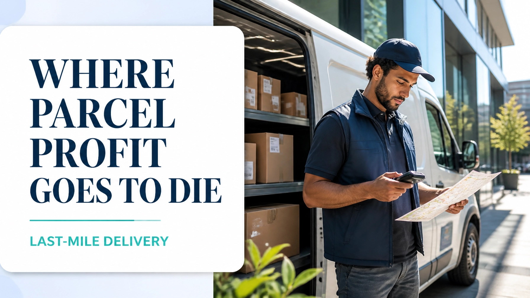
In the realm of logistics, the final leg from local sortation centre to customer doorstep is where service promises become operational reality. It is also where cost, variation and customer-facing failure accumulate quickly.
A parcel may travel efficiently across a national network, only to lose margin through a poorly sequenced route, an unavailable customer, an inaccurate address, excessive parking time or a return-to-depot loop. Last-mile delivery is usually the most labour-intensive, variable and difficult-to-standardise stage of the supply chain because every stop has different access conditions, traffic patterns, customer behaviours and delivery constraints.
This is precisely why value stream mapping is valuable in courier operations. Rather than examining delivery performance through isolated metrics, a value stream map follows the complete parcel journey, including physical movement and information flow. It reveals where time is added, where decisions are delayed, where defects trigger rework and where capacity is consumed without creating customer value.
For a practical overview of the broader method, see this guide to Value Stream Mapping. The same principles apply in last-mile delivery, but the map must include route execution, delivery attempts, exceptions and returns.
Why Last-Mile Delivery Consumes Margin
The customer typically defines value as:
- The correct parcel
- Delivered to the correct location
- Within the promised time window
- In acceptable condition
- With accurate and timely status updates
Everything else should be questioned. Some activities are necessary but non-value-adding, such as security checks or statutory scanning. Others are pure waste: searching for parcels, waiting for access, driving unnecessary kilometres, correcting address errors or attempting delivery without a reasonable probability of success.
The fundamental purpose of a last-mile value stream map is therefore to compare customer value, operational effort and commercial cost across the entire journey.
A useful scope might begin when parcels arrive at a local depot and end when they are:
- Delivered successfully on the first attempt.
- Redirected to an alternative location.
- Reattempted on a later route.
- Returned to the depot or sender.
The information stream must be mapped alongside the parcel. Include order data, address quality, route instructions, customer notifications, proof of delivery, exception codes and return authorisations.

How to Map a Parcel Journey from Sortation to Doorstep
A current-state map should describe what actually happens: not what the standard operating procedure says should happen.
Walk the process with a driver, dispatcher and depot team. Follow representative parcels across different route types, including dense urban, suburban and low-density regional routes.
Capture these stages:
-
Inbound scan and sortation
Record arrival time, scan completion, route assignment and the number of parcels requiring manual handling. -
Route planning and dispatch
Document when routes are created, what data is used, how late orders are handled and whether dispatchers can change the plan after departure. -
Vehicle loading
Measure loading duration, search time, misloads, parcel sequence accuracy and departure readiness. -
Travel to the first delivery zone
Record planned versus actual travel time and kilometres, including congestion, depot exit delays and route deviations. -
Stop-level execution
Measure parking, walking, customer contact, verification, proof-of-delivery capture and departure time. -
Exception handling
Categorise failed attempts by cause: customer unavailable, access problem, inaccurate address, damaged parcel, vehicle capacity issue or driver decision. -
Reattempt, collection or return
Track how failed parcels are held, re-sorted, reallocated and reintroduced into the delivery stream. -
Closeout and performance reporting
Capture end-of-route scanning, cash or device reconciliation, damage reporting and manual administration.
For each step, record processing time, waiting time, queue size, first-pass yield, failure rate, handoffs and information defects. In a service process, value-added time is not limited to physical handling. A correctly executed delivery confirmation can create value because it completes the customer promise. Searching for an address or re-entering information does not.
Worked Example: A Suburban Courier Route
Consider a hypothetical suburban parcel route measured over 20 operating days.
The route carries 92 parcels across 78 delivery stops. The driver has a nine-hour shift, including a 30-minute break.
Current-state measurements
- Planned route distance: 64 kilometres
- Actual route distance: 81 kilometres
- Planned delivery time: 7 hours 15 minutes
- Actual route execution time: 8 hours 5 minutes
- Average stops per hour: 9.6
- Average dwell time per stop: 4.7 minutes
- First-attempt delivery success: 86%
- Failed delivery attempts: 11 of 78 stops
- Average customer waiting or access delay at failed stops: 8.5 minutes
- Return-to-depot volume: 13 parcels per day
- Misloaded or incorrectly sequenced parcels: 4 parcels per day
- Route planning and dispatch preparation: 52 minutes
- Vehicle loading: 38 minutes
- Depot departure delay: 17 minutes
The route appears productive because it completes 92 parcels. However, the map shows that only 67 stops are completed successfully on the first attempt. The remaining 11 failed stops create rework, additional customer communication, re-routing and future depot inventory.
The difference between planned and actual distance is also significant: 17 unnecessary kilometres per route, or approximately 340 kilometres over 20 operating days. At an assumed operating cost of $0.85 per kilometre, that represents $289 in avoidable monthly route expense for one route, before labour, fuel escalation, vehicle depreciation or customer service costs are considered.
The direct financial impact is only part of the problem. Failed deliveries consume future route capacity. If each reattempt requires 6.5 minutes of stop time and 4 minutes of additional travel and handling, 11 failures create approximately:
11 × 10.5 minutes = 115.5 minutes of recurring rework capacity
That is almost two hours of additional work generated by one route’s daily failure pattern.
The Eight Wastes in Route Execution and Dispatch
The eight DOWNTIME wastes provide a disciplined way to classify findings.
- Defects: Incorrect addresses, damaged parcels, failed scans, misloads and inaccurate delivery instructions.
- Overproduction: Sending duplicate notifications, creating unnecessary reattempt tasks or dispatching parcels before customer availability is confirmed.
- Waiting: Drivers waiting for loading completion, access, customer responses, dispatch instructions or route recalculation.
- Non-utilised talent: Ignoring driver knowledge about building access, parking patterns, recurring address issues and practical route constraints.
- Transportation: Excess kilometres caused by backtracking, poor sequencing, depot returns and avoidable reattempt travel.
- Inventory: Parcels held at the depot, in vehicles or in exception cages awaiting a decision.
- Motion: Repeated walking, searching, lifting, device handling and movement between poorly sequenced parcels.
- Extra-processing: Duplicate scans, manual address research, repeated data entry and excessive approval steps for routine exceptions.
These wastes interact. A defective address creates waiting. Waiting causes route delay. Route delay increases failed deliveries. Failed deliveries generate inventory and transportation waste. The map makes this chain visible.
Designing the Future State: Density, Dynamic Routing and Precision
A future-state map should not simply call for “more technology.” It should show how better information changes the flow of work.
For the example route, the improvement team could introduce:
- Dynamic routing: Recalculate sequences using live traffic, new delivery priorities, failed-attempt information and driver progress.
- Delivery-density analysis: Group stops by geographic proximity and building access patterns rather than relying solely on fixed territory boundaries.
- Customer time-slot precision: Offer narrower, more credible delivery windows based on route capacity and historical arrival data.
- Pre-delivery confirmation: Prompt customers to confirm availability, nominate a safe place or select a locker before the vehicle reaches the stop.
- Load sequencing: Place parcels in vehicle order using route clusters, reducing search and unnecessary motion.
- Exception standardisation: Use defined codes and response rules for access issues, address defects and customer unavailability.
- Daily route segmentation: Compare performance by stops per kilometre, parcels per stop, density band and building type.
The target is not merely faster driving. It is more successful deliveries per kilometre and per labour hour.

Current-State Versus Future-State Metrics
| Metric | Current state | Future-state target | Improvement |
|---|---|---|---|
| Parcels per route | 92 | 96 | +4.3% |
| Delivery stops per hour | 9.6 | 11.2 | +16.7% |
| Average dwell time per stop | 4.7 min | 3.9 min | -17.0% |
| First-attempt delivery success | 86% | 94% | +8 percentage points |
| Failed stops per route | 11 | 5 | -54.5% |
| Actual route distance | 81 km | 69 km | -14.8% |
| Route preparation time | 52 min | 32 min | -38.5% |
| Misloaded parcels per day | 4 | 1 | -75.0% |
| Return-to-depot parcels | 13 | 6 | -53.8% |
| Route completion time | 8 h 5 min | 7 h 20 min | -45 min |
These are illustrative targets, not universal benchmarks. Each organisation should establish its own baseline using reliable route, scan, customer and cost data.
Running a Kaizen Event with Drivers and Dispatchers
A last-mile improvement event should include the people who experience the process at ground level. Drivers know where maps fail, which buildings have access delays and which customer instructions are unreliable. Dispatchers understand cut-off pressures, route balancing and exception escalation. Their knowledge is operational data.
A focused three-day kaizen event could follow this structure:
Day 1: Observe and define
- Confirm the value stream scope.
- Walk the depot and observe loading.
- Ride along on representative routes.
- Build the current-state map.
- Agree on operational definitions for failure, dwell time, reattempt and successful delivery.
Day 2: Analyse and prioritise
- Segment performance by route density and delivery type.
- Create a Pareto chart of failed-delivery causes.
- Use a process cycle efficiency calculation to distinguish processing from waiting.
- Identify bottlenecks using route capacity, depot queues and stop-level time.
- Test root causes with drivers, dispatchers and customer service staff.
Day 3: Design and test
- Draw the future-state map.
- Select low-risk countermeasures.
- Run a controlled pilot on two comparable routes.
- Define owners, measures and review dates.
- Establish a daily control board for first-attempt success, kilometres, dwell time and returns.
This approach aligns naturally with DMAIC project practice. Define the delivery problem, measure the actual stream, analyse root causes, improve the flow and control the gains through visual management and standard work.

Control the Gains with the Right Measures
A future state is only useful if performance remains visible after the project team leaves.
Track a balanced set of measures:
- First-attempt delivery success
- On-time delivery percentage
- Stops per hour
- Parcels per kilometre
- Average dwell time
- Planned versus actual route distance
- Failed-attempt reason codes
- Return-to-depot volume
- Route preparation time
- Customer contact rate
- Driver overtime
- Cost per successful delivery
Avoid optimising one metric at the expense of the system. Increasing parcels per route may reduce cost per parcel but damage first-attempt success if the route becomes overloaded. Reducing kilometres may increase dwell time if the revised sequence creates difficult access patterns. The correct goal is reliable, defect-free flow at the lowest total cost.
Build the Capability to Improve Logistics Processes
Value stream mapping gives courier organisations a shared view of where parcel profit is lost. It connects customer expectations with route data, depot constraints, human expertise and financial outcomes.
For professionals working in logistics, operations, dispatch, fulfilment or continuous improvement, Lean Six Sigma training provides the structured problem-solving capability required to turn observations into measurable results. A Lean Six Sigma Green Belt programme can help you apply DMAIC, process mapping, root-cause analysis, statistical tools and control methods to real operational challenges.
Pursue Lean Six Sigma certification and learn how to map, analyse and improve the value streams that determine delivery performance and profitability.
Kaizen. Kai-Care. Kai-Done. ( Lean Six Sigma)